7: Normal Distributions
7: Normal DistributionsObjectives
- Describe the standard normal distribution
- Determine the area under a normal distribution using Minitab
- Determine the points that offset a given proportion of a normal distribution using Minitab
- Summarize the Central Limit Theorem
- Conducted a hypothesis test using a standardized test statistic
- Construct a confidence interval using the standard form
Over the last three lessons you have approximated sampling distributions using bootstrapping and randomization methods. You may have noticed that many of the distributions that you constructed had similar shapes, such as those below:
Randomization Dotplot of Proportion
Bootstrap Dotplot of Mean
Bootstrap Dotplot of Correlation
Randomization Dotplot of \(\bar{x}_1-\bar{x}_2\)
These are all approximately normally distributed. You were first introduced to the normal distribution in Lesson 2 as a special type of symmetrical distribution. In this lesson, we'll review normal distributions, learn how to use Minitab to construct plots of normal distributions, and learn how the Central Limit Theorem allows us to apply what we know about the normal distribution to construct confidence intervals and conduct hypothesis tests without using simulations.
7.1 - Standard Normal Distribution
7.1 - Standard Normal DistributionA normal distribution is a bell-shaped distribution. Theoretically, a normal distribution is continuous and may be depicted as a density curve, such as the one below. The distribution plot below is a standard normal distribution. A standard normal distribution has a mean of 0 and standard deviation of 1. This is also known as the z distribution. You may see the notation \(N(\mu, \sigma\)) where N signifies that the distribution is normal, \(\mu\) is the mean of the distribution, and \(\sigma\) is the standard deviation of the distribution. A z distribution may be described as \(N(0,1)\).
While we cannot determine the probability for any one given value because the distribution is continuous, we can determine the probability for a given interval of values. The probability for an interval is equal to the area under the density curve. The total area under the curve is 1.00, or 100%. In other words, 100% of observations fall under the curve.
For example, in Lesson 2 we learned about the Empirical Rule which stated that approximately 68% of observations on a normal distribution will fall within one standard deviation of the mean, approximately 95% will fall within two standard deviations of the mean, and approximately 99.7% will fall within three standard deviations of the mean.
Example: SAT-Math Scores
The distribution of SAT-Math scores can be described as \(N(500, 100)\). Let's apply the Empirical Rule to determine the SAT-Math scores that separate the middle 68% of scores, the middle 95% of scores, and the middle 99.7% of scores.
Middle 68%: \(500\pm1(100)=[400, 600]\)
Middle 95%: \(500\pm2(100)=[300, 700]\)
Middle 99.7%: \(500\pm 3(100)= [200, 800]\)
z scores
In Lesson 2 we wanted to describe one observation in relation to the distribution of all observations. We did this using a z score.
- z score
-
Distance between an individual score and the mean in standard deviation units; also known as a standardized score.
- z score
- \(z=\dfrac{x - \overline{x}}{s}\)
-
\(x\) = original data value
\(\overline{x}\) = mean of the original distribution
\(s\) = standard deviation of the original distribution
This equation could also be rewritten in terms of population values: \(z=\dfrac{x-\mu}{\sigma}\)
Example: IQ Scores
IQ scores are normally distributed with a mean of 100 and standard deviation of 15. Compute the z score for an individual with an IQ score of 120.
\(z=\dfrac{x- \mu}{\sigma}\)
Here, \(x=120\), \(\mu=100\), and \(\sigma=15\).
\(z=\dfrac{120-100}{15}=\dfrac{20}{15}=1.333\)
This individual's z score is 1.333. Their IQ is 1.333 standard deviations above the mean.
7.2 - Minitab: Finding Proportions Under a Normal Distribution
7.2 - Minitab: Finding Proportions Under a Normal DistributionMinitab can be used to find the proportion of a normal distribution in a given range. The default in Minitab is to construct a standard normal distribution (i.e., z distribution), but the mean and standard deviation of the distribution can be edited. The following pages walk through how to construct normal distributions to find the proportion greater than a given value, the proportion less than a given value, or the proportion between two given values.
Later in this lesson, we'll see that these procedures may be used to find the p value for a given test statistic. For a right-tailed test, the p value is the area greater than the test statistic. For a left-tailed test the p value is the area less than the test statistic. For a two-tailed test, the p value is the total area in the left and right tails that is more extreme than the test statistic.
7.2.1 - Proportion 'Less Than'
7.2.1 - Proportion 'Less Than'The cumulative probability for a value is the probability less than or equal to that value. In notation, this is \(P(X\leq x)\). The proportion at or below a given value is also known as a percentile.
Minitab® – Proportion Less Than a z Value
Question: What proportion of the standard normal distribution is less than a z score of -2?
Recall that the standard normal distribution (i.e., z distribution) has a mean of 0 and standard deviation of 1. This is the default normal distribution in Minitab.
- From the tool bar select Graph > Probability Distribution Plot > One Curve > View Probability
- Check that the Mean is 0 and the Standard deviation is 1
- Select Options
- Select A specified x value
- Select Left tail
- For X value enter -2
- Click Ok
- Click Ok
This should result in the following output:
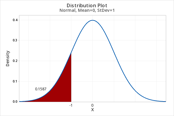
The proportion of the standard normal distribution that is less than a z score of -2 is 0.02275.
This could also be written as P(z < -2) = 0.02275.
Minitab® – Proportion Less Than a Value on a Normal Distribution
Scenario: Vehicle speeds at a highway location have a normal distribution with a mean of 65 mph and a standard deviation of 5 mph. What is the probability that a randomly selected vehicle will be going 73 mph or slower?
Let's construct a normal distribution with a mean of 65 and standard deviation of 5 to find the area less than 73.
- From the tool bar select Graph > Probability Distribution Plot > One Curve > View Probability
- Change the Mean to 65 and the Standard deviation to 5
- Select Options
- Select A specified x value
- Select Left tail
- For X value enter 73
- Click Ok
- Click Ok
This should result in the following output:
On a normal distribution with a mean of 65 mph and standard deviation of 5 mph, the proportion less than 73 mph is 0.9452.
In other words, 94.52% of vehicles will be going 73 mph or slower.
7.2.1.1 - Example: P(Z<-1)
7.2.1.1 - Example: P(Z<-1)Question: What proportion of the z distribution falls below a z score of -1?
- In Minitab select Graph > Probability Distribution Plot > One Curve > View Probability, hit OK.
- Select Normal (Note: The default is the standard normal distribution)
- Select Options
- Select A specified x value
- Select Left Tail
- For X value enter -1
- OK
7.2.1.2 - Example: P(SATM<540)
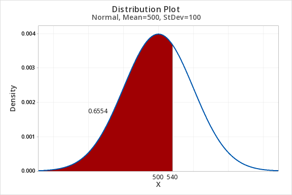
7.2.1.2 - Example: P(SATM<540)Question: SAT-Math scores are normally distributed with a mean of 500 and standard deviation of 100. What proportion of scores are less than 540?
- In Minitab choose Graph > Probability Distribution Plot > View Probability
- For Distribution select Normal (Note: This is the default)
- For Mean enter 500
- For Standard deviation enter 100
- Select Options
- Select A specified X value
- Select Left tail
- For X value enter 540
The proportion of scores less than 540 is 0.6554.
7.2.2 - Proportion 'Greater Than'
7.2.2 - Proportion 'Greater Than'The following two examples use Minitab to find the area under a normal distribution that is greater than a given value. The first example uses the standard normal distribution (i.e., z distribution), which has a mean of 0 and standard deviation of 1; this is the default when first constructing a probability distribution plot in Minitab. The second example models a normal distribution with a mean of 65 and standard deviation of 5.
Later in this lesson we'll see that these methods can be used to identify p values when conducting right-tailed hypothesis tests.
Minitab® – Proportion Greater Than a Value on a Normal Distribution
Question: What proportion of the standard normal distribution is greater than a z score of 2?
Recall that the standard normal distribution (i.e., z distribution) has a mean of 0 and standard deviation of 1. This is the default normal distribution in Minitab.
- From the tool bar select Graph > Probability Distribution Plot > One Curve > View Probability
- Check that the Mean is 0 and the Standard deviation is 1
- Select Options
- Select A specified x value
- Select Right tail
- For X value enter 2
- Click Ok
- Click Ok
This should result in the following output:
The area of the z distribution that is greater than 2 is 0.02275.
This could also be written in probability notation as P(z > 2) = 0.02275.
Minitab® – Proportion Greater Than a Value on a Normal Distribution
Question: Vehicle speeds at a highway location have a normal distribution with a mean of 65 mph and a standard deviation of 5 mph. What is the probability that a randomly selected vehicle will be going more than 73 mph?
Let's construct a normal distribution with a mean of 65 and standard deviation of 5 to find the area greater than 73.
To calculate a probability for values greater than a given value in Minitab:
- From the tool bar select Graph > Probability Distribution Plot > One Curve > View Probability
- Change the Mean to 65 and the Standard deviation to 5
- Select Options
- Select A specified x value
- Select Right tail
- For X value enter 73
- Click Ok
- Click Ok
This should result in the following output:
On a normal distribution with a mean of 65 and standard deviation of 5, the proportion greater than 73 is 0.05480.
In other words, 5.480% of vehicles will be going more than 73 mph.
7.2.2.1 - Example: P(Z>0.5)
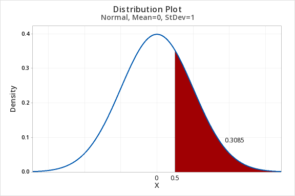
7.2.2.1 - Example: P(Z>0.5)Question: What proportion of the z distribution is greater than z = 0.5?
- In Minitab select Graph > Probability Distribution Plot > One Curve > View Probability, hit OK.
- Select Normal and enter 0 for the mean and 1 for the standard deviation.(Note: The default is the standard normal distribution)
- Select Options
- Select A specified x value
- Select Right Tail
- For X value enter 0.5
- Click OK
7.2.3 - Proportion 'In between'
7.2.3 - Proportion 'In between'In the following examples we will use Minitab to find the area under a normal distribution between two values. The first example uses the z distribution and the second example uses a normal distribution with a mean of 65 and standard deviation of 5.
Minitab® – Area Between Two z Values
Question: What proportion of the standard normal distribution is between a z score of 0 and a z score of 1.75?
Recall that the standard normal distribution (i.e., z distribution) has a mean of 0 and standard deviation of 1. This is the default normal distribution in Minitab.
- From the tool bar select Graph > Probability Distribution Plot > One Curve > View Probability
- Check that the Mean is 0 and the Standard deviation is 1
- Select Options
- Select A specified x value
- Select Middle
- For X value 1 enter 0
- For X value 2 enter 1.75
- Click Ok
- Click Ok
This should result in the following output:
The proportion of the z distribution that is between 0 and 1.75 is 0.4599.
In probability notation, this could be written as P(0 ≤ z ≤ 1.75) = 0.4599
Minitab®
Area Between Two Values on a Normal Distribution
Question: Vehicle speeds at a highway location have a normal distribution with a mean of 65 mph and a standard deviation of 5 mph. What is the probability that a randomly selected vehicle will be going between 60 mph and 73 mph?
Let's construct a normal distribution with a mean of 65 and standard deviation of 5 to find the area between 60 and 73.
- From the tool bar select Graph > Probability Distribution Plot > One Curve > View Probability
- Change the Mean to 65 and the Standard deviation to 5
- Select Options
- Select A specified x value
- Select Middle
- For X value 1 enter 60
- For X value 2 enter 73
- Click Ok
- Click Ok
This should result in the following output:
On a normal distribution with a mean of 65 mph and standard deviation of 5 mph, the proportion of observations between 60 mph and 73 mph is 0.7865.
In other words, 78.65% of vehicles will be going between 60 mph and 73 mph.
7.2.3.1 - Example: Proportion Between z -2 and +2
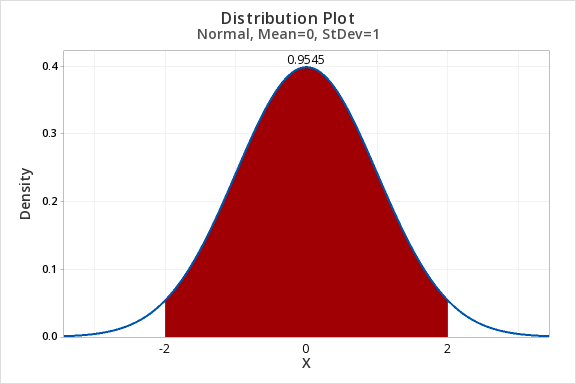
7.2.3.1 - Example: Proportion Between z -2 and +2Question: What proportion of the z distribution is between -2 and 2?
- In Minitab select Graph > Probability Distribution Plot > One Curve > View Probability, hit OK.
- Select Normal and enter 0 for the mean and 1 for the standard deviation.(Note: The default is the standard normal distribution)
- Select Options
- Select A specified x value
- Select Middle and enter
- X value 1: -2
- X value 2: 2
- Select OK
7.2.4 - Proportion 'More Extreme Than'
7.2.4 - Proportion 'More Extreme Than'Minitab® – Proportion More Extreme than a z Score
Question: What proportion of the standard normal distribution is more extreme than a z value of ±2?
- From the tool bar select Graph > Probability Distribution Plot > One Curve > View Probability
- Check that the Mean is 0 and the Standard deviation is 1
- Select Options
- Select A specified x value
- Select Equal Tails
- For X value enter 2 or -2*
- Click Ok
- Click Ok
* By default, "equal tails" will result in a symmetric distribution. In other words, the same proportion will be in the left and right tails.
This should result in the following output:
To find the total proportion of the z distribution that is more extreme than a z value of ±2 we need to add together the area in the two tails:
0.02275 + 0.02275 = 0.0455
The area that is more than two standard deviations from the mean on a normal distribution is 0.0455, or 4.55%.
Minitab®
Question: Vehicle speeds at a highway location have a normal distribution with a mean of 65 mph and a standard deviation of 5 mph. What proportion of vehicles are deviating from the mean by 10 mph or more? In other words, what proportion are going less than 55 mph or more than 75 mph?
Let's construct a normal distribution with a mean of 65 and standard deviation of 5 to find the area more than 10 mph from the mean.
- From the tool bar select Graph > Probability Distribution Plot > One Curve > View Probability
- Change the Mean to 65 and the Standard deviation to 5
- Select Options
- Select A specified x value
- Select Equal Tails
- For X value enter 55 or 75*
- Click Ok
- Click Ok
* By default, "equal tails" will result in a symmetric distribution. In other words, the same proportion will be in the left and right tails.
This should result in the following output:
To find the total proportion of vehicles that are deviating from the mean by 10 mph or more we need to add together the area in the two tails:
0.02275 + 0.02275 = 0.0455
The proportion of vehicles deviating from the mean by 10 mph or more is 0.0455, or 4.55%.
7.3 - Minitab: Finding Values Given Proportions
7.3 - Minitab: Finding Values Given ProportionsMinitab can also be used to find the values that separate a given proportion of the normal distribution. This can be used to find the value that offset a given proportion, such as the top 10%, bottom 25%, or middle 95%. In this lesson, we'll learn how to find such values on the z distribution or on a normal distribution with a given mean and standard deviation.
In Lesson 4, we used the standard error method to construct a 95% confidence interval by estimating the z* multiplier to be 2 using the Empirical Rule, because approximately 95% of a normal distribution falls within two standard deviations of the mean. Later in this lesson, we'll see that the procedures we're learning here, specifically finding the z scores that offset the middle X%, can be used to determine the z* multiplier to construct a confidence interval for any confidence level. For example, we can use Minitab to find the z values that offset the middle 90% of the z distribution, which would be the multipliers for a 90% confidence interval.
7.3.1 - Top X%
7.3.1 - Top X%On this page, we'll focus on finding the values that offset the top X% of a normal distribution, for example the top 10% or top 20%. The first example below uses the standard normal distribution. The second exam uses a normal distribution with a mean of 85 and standard deviation of 5.
Minitab® – z Score Separating the Top X%
Question: What z score separates the top 10% of the z distribution from the bottom 90%?
- From the tool bar select Graph > Probability Distribution Plot > One Curve > View Probability
- Check that the Mean is 0 and the Standard deviation is 1
- Select Options
- Select A specified probability
- Select Right tail
- For Probability enter 0.10
- Click Ok
- Click Ok
This should result in the following output:
A z score of 1.282 separates the top 10% of the z distribution from the bottom 90%.
Minitab® – Value Separating the Top X%
Question: Scores on a test are normally distributed with a mean of 85 points and standard deviation of 5 points. What score separates the top 10% from the bottom 90%?
- From the tool bar select Graph > Probability Distribution Plot > One Curve > View Probability
- Change the Mean to 85 and the Standard deviation to 5
- Select Options
- Select A specified probability
- Select Right tail
- For Probability enter 0.10
- Click Ok
- Click Ok
This should result in the following output:
The test score that separates the top 10% from the bottom 90% is 91.41 points. This could also be described as the 90th percentile.
7.3.2 - Bottom X%
7.3.2 - Bottom X%Next, we'll find the z scores or observations that off set the bottom X% of a normal distribution. Earlier in this lesson, we learned that this is also known as the cumulative proportion or percentile. The first example below uses the z distribution. The second example uses a normal distribution with a mean of 85 and standard deviation of 5.
Minitab® – z Score Separating the Bottom X%
Question: What z score separates the bottom 10% of the standard normal distribution from the top 90%?
- From the tool bar select Graph > Probability Distribution Plot > One Curve > View Probability
- Check that the Mean is 0 and the Standard deviation is 1
- Select Options
- Select A specified probability
- Select Left tail
- For Probability enter 0.10
- Click Ok
- Click Ok
This should result in the following output:
A z score of -1.282 separates the bottom 10% of the z distribution from the top 90%.
Minitab® – Value on a Normal Distribution Separating the Bottom X%
Question: Scores on a test are normally distributed with a mean of 85 points and standard deviation of 5 points. What score is the 10th percentile? In other words, what score separates the bottom 10% from the top 90% of this distribution?
- From the tool bar select Graph > Probability Distribution Plot > One Curve > View Probability
- Change the Mean to 85 and the Standard deviation to 5
- Select Options
- Select A specified probability
- Select Left tail
- For Probability enter 0.10
- Click Ok
- Click Ok
This should result in the following output:
The 10th percentile on this test is a score of 78.59 points.
7.3.3 - Middle X%
7.3.3 - Middle X%Here, we'll use Minitab to find the points on a normal distribution that offset the most extreme X%. The first example below uses the z distribution, which later in the lesson we'll see can be plugged into the formula for a confidence interval to obtain an interval with any confidence level. For example, the z scores that separate the middle 90% from the outer 10% could be used to compute a 90% confidence interval. The second example below is similar, but it uses a distribution with a mean of 85 and standard deviation of 5.
Note that in Minitab, the proportion you will enter is the total proportion in the two tails combined. Minitab will split that proportion equally between the left and right tails.
Minitab® – z Scores Separating the Middle X%
Question: What z scores separate the middle 90% of the z distribution from the most extreme 10%?
- From the tool bar select Graph > Probability Distribution Plot > One Curve > View Probability
- Check that the Mean is 0 and the Standard deviation is 1
- Select Options
- Select A specified probability
- Select Equal tails
- For Probability enter 0.10
- Click Ok
- Click Ok
This should result in the following output:
The z scores of ±1.645 separate the middle 90% of the z distribution from the outer 10% .
Minitab® – Values on a Normal Distribution Separating the Middle X%
Question: Scores on a test are normally distributed with a mean of 85 points and standard deviation of 5 points. What scores separate the middle 90% from the most extreme 10%?
- From the tool bar select Graph > Probability Distribution Plot > One Curve > View Probability
- Change the Mean to 85 and the Standard deviation to 5
- Select Options
- Select A specified probability
- Select Equal tails
- For Probability enter 0.10
- Click Ok
- Click Ok
This should result in the following output:
The middle 90% of scores are between 76.78 points and 93.22 points.
7.4 - Central Limit Theorem
7.4 - Central Limit TheoremAs we saw at the beginning of this lesson, many of the sampling distributions that you have constructed and worked with this semester are approximately normally distributed. The reason behind this is one of the most important theorems in statistics.
Central Limit Theorem
The Central Limit Theorem states that if the sample size is sufficiently large then the sampling distribution will be approximately normally distributed for many frequently tested statistics, such as those that we have been working with in this course: one sample mean, one sample proportion, difference in two means, difference in two proportions, the slope of a simple linear regression model, and Pearson's r correlation.
Over the next few lessons we will examine what constitutes a "sufficiently large" sample size. Essentially, it is determined by the point at which the sampling distribution becomes approximately normal.
In practice, when we construct confidence intervals and conduct hypothesis tests we often use the normal distribution (or t distributions which you'll see next week) as opposed to bootstrapping or randomization procedures in situations when the sampling distribution is approximately normal. This method is preferred by many because z scores are on a standard scale (i.e., mean of 0 and standard deviation of 1) which makes interpreting results more straight forward.
Drag the slider at the bottom of the graph to see normal curve fit on the randomization plot.
7.4.1 - Hypothesis Testing
7.4.1 - Hypothesis TestingFive Step Hypothesis Testing Procedure
In the remaining lessons, we will use the following five step hypothesis testing procedure. This is slightly different from the five step procedure that we used when conducting randomization tests.
- Check assumptions and write hypotheses. The assumptions will vary depending on the test. In this lesson we'll be confirming that the sampling distribution is approximately normal by visually examining the randomization distribution. In later lessons you'll learn more objective assumptions. The null and alternative hypotheses will always be written in terms of population parameters; the null hypothesis will always contain the equality (i.e., \(=\)).
- Calculate the test statistic. Here, we'll be using the formula below for the general form of the test statistic.
- Determine the p-value. The p-value is the area under the standard normal distribution that is more extreme than the test statistic in the direction of the alternative hypothesis.
- Make a decision. If \(p \leq \alpha\) reject the null hypothesis. If \(p>\alpha\) fail to reject the null hypothesis.
- State a "real world" conclusion. Based on your decision in step 4, write a conclusion in terms of the original research question.
General Form of a Test Statistic
When using a standard normal distribution (i.e., z distribution), the test statistic is the standardized value that is the boundary of the p-value. Recall the formula for a z score: \(z=\frac{x-\overline x}{s}\). The formula for a test statistic will be similar. When conducting a hypothesis test the sampling distribution will be centered on the null parameter and the standard deviation is known as the standard error.
- General Form of a Test Statistic
- \(test\;statistic=\dfrac{sample\;statistic-null\;parameter}{standard\;error}\)
This formula puts our observed sample statistic on a standard scale (e.g., z distribution). A z score tells us where a score lies on a normal distribution in standard deviation units. The test statistic tells us where our sample statistic falls on the sampling distribution in standard error units.
7.4.1.1 - Video Example: Mean Body Temperature
7.4.1.1 - Video Example: Mean Body TemperatureResearch question: Is the mean body temperature in the population different from 98.6° Fahrenheit?
7.4.1.2 - Video Example: Correlation Between Printer Price and PPM
7.4.1.2 - Video Example: Correlation Between Printer Price and PPMResearch question: Is there a positive correlation in the population between the price of an ink jet printer and how many pages per minute (ppm) it prints?
7.4.1.3 - Example: Proportion NFL Coin Toss Wins
7.4.1.3 - Example: Proportion NFL Coin Toss WinsResearch question: Is the proportion of NFL overtime coin tosses that are won different from 0.50?
StatKey was used to construct a randomization distribution:
Step 1: Check assumptions and write hypotheses
From the given StatKey output, the randomization distribution is approximately normal.
\(H_0\colon p=0.50\)
\(H_a\colon p \ne 0.50\)
Step 2: Calculate the test statistic
\(test\;statistic=\dfrac{sample\;statistic-null\;parameter}{standard\;error}\)
The sample statistic is the proportion in the original sample, 0.561. The null parameter is 0.50. And, the standard error is 0.024.
\(test\;statistic=\dfrac{0.561-0.50}{0.024}=\dfrac{0.061}{0.024}=2.542\)
Step 3: Determine the p value
The p value will be the area on the z distribution that is more extreme than the test statistic of 2.542, in the direction of the alternative hypothesis. This is a two-tailed test:
The p value is the area in the left and right tails combined: \(p=0.0055110+0.0055110=0.011022\)
Step 4: Make a decision
The p value (0.011022) is less than the standard 0.05 alpha level, therefore we reject the null hypothesis.
Step 5: State a "real world" conclusion
There is evidence that the proportion of all NFL overtime coin tosses that are won is different from 0.50
7.4.1.4 - Example: Proportion of Women Students
7.4.1.4 - Example: Proportion of Women StudentsResearch question: Are more than 50% of all World Campus STAT 200 students women?
Data were collected from a representative sample of 501 World Campus STAT 200 students. In that sample, 284 students were women and 217 were not women.
StatKey was used to construct a sampling distribution using randomization methods:
Because this randomization distribution is approximately normal, we can find the p value by computing a standardized test statistic and using the z distribution.
Step 1: Check assumptions and write hypotheses
The assumption here is that the sampling distribution is approximately normal. From the given StatKey output, the randomization distribution is approximately normal.
\(H_0\colon p=0.50\)
\(H_a\colon p>0.50\)
2. Calculate the test statistic
\(test\;statistic=\dfrac{sample\;statistic-hypothesized\;parameter}{standard\;error}\)
The sample statistic is \(\widehat p = 284/501 = 0.567\).
The hypothesized parameter is the value from the hypotheses: \(p_0=0.50\).
The standard error on the randomization distribution above is 0.022.
\(test\;statistic=\dfrac{0.567-0.50}{0.022}=3.045\)
3. Determine the p value
We can find the p value by constructing a standard normal distribution and finding the area under the curve that is more extreme than our observed test statistic of 3.045, in the direction of the alternative hypothesis. In other words, \(P(z>3.045)\):
Our p value is 0.0011634
4. Make a decision
Our p value is less than or equal to the standard 0.05 alpha level, therefore we reject the null hypothesis.
5. State a "real world" conclusion
There is evidence that the proportion of all World Campus STAT 200 students who are women is greater than 0.50.
7.4.1.5 - Example: Mean Quiz Score
7.4.1.5 - Example: Mean Quiz ScoreResearch question: Is the mean quiz score different from 14 in the population?
StatKey was used to construct a randomization distribution:
Step 1: Check assumptions and write hypotheses
From the given StatKey output, the randomization distribution is approximately normal.
\(H_0\colon \mu = 14\)
\(H_a\colon \mu \ne 14\)
Step 2: Calculate the test statistic
\(test\;statistic=\dfrac{sample\;statistic-null\;parameter}{standard\;error}\)
The sample statistic is the mean in the original sample, 13.746 points. The null parameter is 14 points. And, the standard error, 0.142, can be found on the StatKey output.
\(test\;statistic=\dfrac{13.746-14}{0.142}=\dfrac{-0.254}{0.142}=-1.789\)
Step 3: Determine the p value
The p value will be the area on the z distribution that is more extreme than the test statistic of -1.789, in the direction of the alternative hypothesis:
This was a two-tailed test. The p value is the area in the left and right tails combined: \(p=0.0368074+0.0368074=0.0736148\)
Step 4: Make a decision
The p value (0.0736148) is greater than the standard 0.05 alpha level, therefore we fail to reject the null hypothesis.
Step 5: State a "real world" conclusion
There is not enough evidence to state that the mean quiz score in the population is different from 14 points.
7.4.1.6 - Example: Difference in Mean Commute Times
7.4.1.6 - Example: Difference in Mean Commute TimesResearch question: Do the mean commute times in Atlanta and St. Louis differ in the population?
StatKey was used to construct a randomization distribution:
Step 1: Check assumptions and write hypotheses
From the given StatKey output, the randomization distribution is approximately normal.
\(H_0: \mu_1-\mu_2=0\)
\(H_a: \mu_1 - \mu_2 \ne 0\)
Step 2: Compute the test statistic
\(test\;statistic=\dfrac{sample\;statistic - null \; parameter}{standard \;error}\)
The observed sample statistic is \(\overline x _1 - \overline x _2 = 7.14\). The null parameter is 0. And, the standard error, from the StatKey output, is 1.136.
\(test\;statistic=\dfrac{7.14-0}{1.136}=6.285\)
Step 3: Determine the p value
The p value will be the area on the z distribution that is more extreme than the test statistic of 6.285, in the direction of the alternative hypothesis:
This was a two-tailed test. The area in the two tailed combined is 0.000000. Theoretically, the p value cannot be 0 because there is always some chance that a Type I error was committed. This p value would be written as p < 0.001.
Step 4: Make a decision
The p value is smaller than the standard 0.05 alpha level, therefore we reject the null hypothesis.
Step 5: State a "real world" conclusion
There is evidence that the mean commute times in Atlanta and St. Louis are different in the population.
7.4.2 - Confidence Intervals
7.4.2 - Confidence IntervalsStandard Normal Distribution Method
The normal distribution can also be used to construct confidence intervals. You used this method when you first learned to construct confidence intervals using the standard error method. Recall the formula you used:
- 95% Confidence Interval
- \(sample\;statistic \pm 2 (standard\;error)\)
The 2 in this formula comes from the normal distribution. According to the 95% Rule, approximately 95% of a normal distribution falls within 2 standard deviations of the mean.
Using the normal distribution, we can conduct a confidence interval for any level using the following general formula:
- General Form of a Confidence Interval
- sample statistic \(\pm\) \(z^*\) (standard error)
- \(z^*\) is the multiplier
The \(z^*\) multiplier can be found by constructing a z distribution in Minitab.
z* Multiplier for a 90% Confidence Interval
What z* multiplier should be used to construct a 90% confidence interval?
For a 90% confidence interval, we would find the z scores that separate the middle 90% of the z distribution from the outer 10% of the z distribution:
For a 90% confidence interval, the \(z^*\) multiplier will be 1.64485.
7.4.2.1 - Video Example: 98% CI for Mean Atlanta Commute Time
7.4.2.1 - Video Example: 98% CI for Mean Atlanta Commute TimeConstruct a 98% confidence interval to estimate the mean commute time in the population of all Atlanta residents.
This example uses a dataset is built in to StatKey: Confidence Interval for a Mean, Median, Std. The dataset is titled 'Atlanta Commute.'
Video Walkthrough
7.4.2.2 - Video Example: 90% CI for the Correlation between Height and Weight
7.4.2.2 - Video Example: 90% CI for the Correlation between Height and WeightConstruct a 90% confidence interval to estimate the correlation between height and weight in the population of all adult men.
Video Walkthrough
7.4.2.3 - Example: 99% CI for Proportion of Women Students
7.4.2.3 - Example: 99% CI for Proportion of Women StudentsScenario: Data were collected from a representative sample of 501 World Campus STAT 200 students. In that sample, 284 students were women and 217 were not women. Construct a 99% confidence interval to estimate the proportion of all World Campus students who are women.
StatKey was used to construct a sampling distribution using bootstrapping methods:
Because this distribution is approximately normal, we can approximate the sampling distribution using the z distribution. We will use the standard error, 0.022, from this distribution.
The original sample statistic was \(\widehat p =\frac{284}{501}=0.567\).
We can find the \(z^*\) multiplier by constructing a z distribution to find the values that separate the middle 99% from the outer 1%:
The \(z^*\) multiplier is 2.57583
Recall the general form of a confidence interval: sample statistic \(\pm\) \(z^*\) (standard error) where \(z^*\) is the multiplier. So in this case we have...
\(0.567 \pm 2.57583 (0.022)\)
\(0.567 \pm 0.057\)
\([0.510, 0.624]\)
I am 99% confident that the proportion of all World Campus students who are women is between 0.510 and 0.624
7.5 - Lesson 7 Summary
7.5 - Lesson 7 SummaryObjectives
- Describe the standard normal distribution
- Determine the area under a normal distribution using Minitab
- Determine the points that offset a given proportion of a normal distribution using Minitab
- Summarize the Central Limit Theorem
- Conduct a hypothesis test using a standardized test statistic
- Construct a confidence interval using the standard form
In this lesson we learned how to find the proportion under a normal distribution. We used the standard normal distribution to approximate the sampling distribution to find p value and to construct confidence intervals. In the next few lessons we will learn about the t distribution, which is similar to the standard normal distribution, and we'll focus more on how Minitab can be used to construct confidence intervals and conduct hypothesis tests using these common distributions.