8.1.2 - Hypothesis Testing
8.1.2 - Hypothesis TestingA hypothesis test for a proportion is used when you are comparing one group to a known or hypothesized population proportion value. In other words, you have one sample with one categorical variable. The hypothesized value of the population proportion is symbolized by \(p_0\) because this is the value in the null hypothesis (\(H_0\)).
If \(np_0 \ge 10\) and \(n(1-p_0) \ge 10\) then the distribution of sample proportions is approximately normal and can be estimated using the normal distribution. That sampling distribution will have a mean of \(p_0\) and a standard deviation (i.e., standard error) of \(\sqrt{\frac{p_0 (1-p_0)}{n}}\)
Recall that the standard normal distribution is also known as the z distribution. Thus, this is known as a "single sample proportion z test" or "one sample proportion z test."
If \(np_0 < 10\) or \(n(1-p_0) < 10\) then the distribution of sample proportions follows a binomial distribution. We will not be conducting this test by hand in this course, however you will learn how this can be conducted using Minitab using the exact method.
8.1.2.1 - Normal Approximation Method Formulas
8.1.2.1 - Normal Approximation Method FormulasHere we will be using the five step hypothesis testing procedure to compare the proportion in one random sample to a specified population proportion using the normal approximation method.
In order to use the normal approximation method, the assumption is that both \(n p_0 \geq 10\) and \(n (1-p_0) \geq 10\). Recall that \(p_0\) is the population proportion in the null hypothesis.
| Research Question | Is the proportion different from \(p_0\)? | Is the proportion greater than \(p_0\)? | Is the proportion less than \(p_0\)? |
|---|---|---|---|
| Null Hypothesis, \(H_{0}\) | \(p=p_0\) | \(p= p_0\) | \(p= p_0\) |
| Alternative Hypothesis, \(H_{a}\) | \(p\neq p_0\) | \(p> p_0\) | \(p< p_0\) |
| Type of Hypothesis Test | Two-tailed, non-directional | Right-tailed, directional | Left-tailed, directional |
Where \(p_0\) is the hypothesized population proportion that you are comparing your sample to.
When using the normal approximation method we will be using a z test statistic. The z test statistic tells us how far our sample proportion is from the hypothesized population proportion in standard error units. Note that this formula follows the basic structure of a test statistic that you learned in the last lesson:
\(test\;statistic=\dfrac{sample\;statistic-null\;parameter}{standard\;error}\)
- Test statistic: One Group Proportion
- \(z=\dfrac{\widehat{p}- p_0 }{\sqrt{\frac{p_0 (1- p_0)}{n}}}\)
-
\(\widehat{p}\) = sample proportion
\(p_{0}\) = hypothesize population proportion
\(n\) = sample size
Given that the null hypothesis is true, the p value is the probability that a randomly selected sample of n would have a sample proportion as different, or more different, than the one in our sample, in the direction of the alternative hypothesis. We can find the p value by mapping the test statistic from step 2 onto the z distribution.
Note that p-values are also symbolized by \(p\). Do not confuse this with the population proportion which shares the same symbol.
We can look up the \(p\)-value using Minitab by constructing the sampling distribution. Because we are using the normal approximation here, we have a \(z\) test statistic that we can map onto the \(z\) distribution. Recall, the z distribution is a normal distribution with a mean of 0 and standard deviation of 1. If we are conducting a one-tailed (i.e., right- or left-tailed) test, we look up the area of the sampling distribution that is beyond our test statistic. If we are conducting a two-tailed (i.e., non-directional) test there is one additional step: we need to multiple the area by two to take into account the possibility of being in the right or left tail.
We can decide between the null and alternative hypotheses by examining our p-value. If \(p \leq \alpha\) reject the null hypothesis. If \(p>\alpha\) fail to reject the null hypothesis. Unless stated otherwise, assume that \(\alpha=.05\).
When we reject the null hypothesis our results are said to be statistically significant.
Based on our decision in step 4, we will write a sentence or two concerning our decision in relation to the original research question.
8.1.2.1.1 - Video Example: Male Babies
8.1.2.1.1 - Video Example: Male Babies8.1.2.1.2 - Example: Handedness
8.1.2.1.2 - Example: HandednessResearch Question: Are more than 80% of American's right handed?
In a sample of 100 Americans, 87 were right handed.
\(np_0 = 100(0.80)=80\)
\(n(1-p_0) = 100 (1-0.80) = 20\)
Both \(np_0\) and \(n(1-p_0)\) are at least 10 so we can use the normal approximation method.
This is a right-tailed test because we want to know if the proportion is greater than 0.80.
\(H_{0}\colon p=0.80\)
\(H_{a}\colon p>0.80\)
Test statistic: One Group Proportion
\(z=\dfrac{\widehat{p}- p_0 }{\sqrt{\frac{p_0 (1- p_0)}{n}}}\)
\(\widehat{p}\) = sample proportion
\(p_{0}\) = hypothesize population proportion
\(n\) = sample size
\(\widehat{p}=\dfrac{87}{100}=0.87\), \(p_{0}=0.80\), \(n=100\)
\(z= \dfrac{\widehat{p}- p_0 }{\sqrt{\frac{p_0 (1- p_0)}{n}}}= \dfrac{0.87-0.80}{\sqrt{\frac{0.80 (1-0.80)}{100}}}=1.75\)
Our \(z\) test statistic is 1.75.
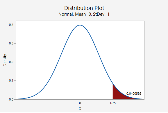
This is a right-tailed test so we need to find the area to the right of the test statistic, \(z=1.75\), on the z distribution.
Using Minitab , we find the probability \(P(z\geq1.75)=0.0400592\) which may be rounded to \(p\; value=0.0401\).
\(p\leq .05\), therefore our decision is to reject the null hypothesis
Yes, there is convincing evidence to state that more than 80% of all Americans are right handed.
8.1.2.1.3 - Example: Ice Cream
8.1.2.1.3 - Example: Ice CreamResearch Question: Is the percentage of Creamery customers who prefer chocolate ice cream over vanilla less than 80%?
In a sample of 50 customers 60% preferred chocolate over vanilla.
\(np_0 = 50(0.80) = 40\)
\(n(1-p_0)=50(1-0.80) = 10\)
Both \(np_0\) and \(n(1-p_0)\) are at least 10. We can use the normal approximation method.
This is a left-tailed test because we want to know if the proportion is less than 0.80.
\(H_{0}\colon p=0.80\)
\(H_{a}\colon p<0.80\)
Test statistic: One Group Proportion
\(z=\dfrac{\widehat{p}- p_0 }{\sqrt{\frac{p_0 (1- p_0)}{n}}}\)
\(\widehat{p}\) = sample proportion
\(p_{0}\) = hypothesize population proportion
\(n\) = sample size
\(\widehat{p}=0.60\), \(p_{0}=0.80\), \(n=50\)
\(z= \dfrac{\widehat{p}- p_0 }{\sqrt{\frac{p_0 (1- p_0)}{n}}}= \dfrac{0.60-0.80}{\sqrt{\frac{0.80 (1-0.80)}{50}}}=-3.536\)
Our \(z\) test statistic is -3.536.
This is a left-tailed test so we need to find the area to the left of our test statistic, \(z=-3.536\).
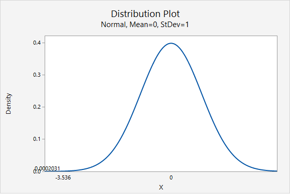
From the Minitab output above, the p-value is 0.0002031
\(p \leq.05\), therefore our decision is to reject the null hypothesis.
Yes, there is convincing evidence that the percentage of all Creamery customers who prefer chocolate ice cream over vanilla is less than 80%.
8.1.2.1.4 - Example: Overweight Citizens
8.1.2.1.4 - Example: Overweight CitizensAccording to the Center for Disease Control (CDC), the percent of adults 20 years of age and over in the United States who are overweight is 69.0% (see http://www.cdc.gov/nchs/fastats/obesity-overweight.htm). One city’s council wants to know if the proportion of overweight citizens in their city is different from this known national proportion. They take a random sample of 150 adults 20 years of age or older in their city and find that 98 are classified as overweight. Let’s use the five step hypothesis testing procedure to determine if there is convincing evidence that the proportion in this city is different from the known national proportion.
\(np_0 =150 (0.690)=103.5 \)
\(n (1-p_0) =150 (1-0.690)=46.5\)
Both \(n p_0\) and \(n (1-p_0)\) are at least 10, this assumption has been met.
Research question: Is this city’s proportion of overweight individuals different from 0.690?
This is a non-directional test because our question states that we are looking for a differences as opposed to a specific direction. This will be a two-tailed test.
\(H_{0}\colon p=0.690\)
\(H_{a}\colon p\neq 0.690\)
Test statistic: One Group Proportion
\(z=\dfrac{\widehat{p}- p_0 }{\sqrt{\frac{p_0 (1- p_0)}{n}}}\)
\(\widehat{p}\) = sample proportion
\(p_{0}\) = hypothesize population proportion
\(n\) = sample size
\(\widehat{p}=\dfrac{98}{150}=.653\)
\( z =\dfrac{0.653- 0.690 }{\sqrt{\frac{0.690 (1- 0.690)}{150}}} = -0.980 \)
Our test statistic is \(z=-0.980\)
This is a non-directional (i.e., two-tailed) test, so we need to find the area under the z distribution that is more extreme than \(z=-0.980\).
In Minitab, we find the proportion of a normal curve beyond \(\pm0.980\):
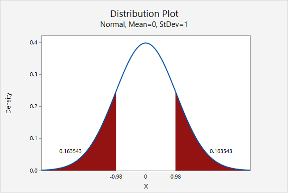
\(p-value=0.163543+0.163543=0.327086\)
\(p>\alpha\), therefore we fail to reject the null hypothesis
There is not sufficient evidence to state that the proportion of citizens of this city who are overweight is different from the national proportion of 0.690.
8.1.2.2 - Minitab: Hypothesis Tests for One Proportion
8.1.2.2 - Minitab: Hypothesis Tests for One ProportionA hypothesis test for one proportion can be conducted in Minitab. This can be done using raw data or summarized data.
- If you have a data file with every individual's observation, then you have raw data.
- If you do not have each individual observation, but rather have the sample size and number of successes in the sample, then you have summarized data.
The next two pages will show you how to use Minitab to conduct this analysis using either raw data or summarized data.
Note that the default method for constructing the sampling distribution in Minitab is to use the exact method. If \(np_0 \geq 10\) and \(n(1-p_0) \geq 10\) then you will need to change this to the normal approximation method. This must be done manually. Minitab will use the method that you select, it will not check assumptions for you!
8.1.2.2.1 - Minitab: 1 Proportion z Test, Raw Data
8.1.2.2.1 - Minitab: 1 Proportion z Test, Raw DataIf you have data in a Minitab worksheet, then you have what we call "raw data." This is in contrast to "summarized data" which you'll see on the next page.
In order to use the normal approximation method both \(np_0 \geq 10\) and \(n(1-p_0) \geq 10\). Before we can conduct our hypothesis test we must check this assumption to determine if the normal approximation method or exact method should be used. This must be checked manually. Minitab will not check assumptions for you.
In the example below, we want to know if there is convincing evidence that the proportion of students who are male is different from 0.50.
\(n=226\) and \(p_0=0.50\)
\(np_0 = 226(0.50)=113\) and \(n(1-p_0) = 226(1-0.50)=113\)
Both \(np_0 \geq 10\) and \(n(1-p_0) \geq 10\) so we can use the normal approximation method.
Minitab® – Conducting a One Sample Proportion z Test: Raw Data
Research question: Is the proportion of students who are male different from 0.50?
- Open Minitab file:
- In Minitab, select Stat > Basic Statistics > 1 Proportion
- Select One or more samples, each in a column from the dropdown
- Double-click the variable Biological Sex to insert it into the box
- Check the box next to Perform hypothesis test and enter 0.50 in the Hypothesized proportion box
- Select Options
- Use the default Alternative hypothesis setting of Proportion ≠ hypothesized proportion value
- Use the default Confidence level of 95
- Select Normal approximation method
- Click OK and OK
The result should be the following output:
Method
Event: Biological Sex = Male
p: proportion where Biological Sex = Male
Normal approximation is used for this analysis.
N | Event | Sample p | 95% CI for p |
|---|---|---|---|
226 | 99 | 0.438053 | (0.373368, 0.502738) |
Null hypothesis | H 0: p = 0.5 |
|---|---|
Alternative hypothesis | H 1: p ≠ 0.5 |
Z-Value | P-Value |
|---|---|
-1.86 | 0.063 |
Summary of Results
We could summarize these results using the five-step hypothesis testing procedure:
\(np_0 = 226(0.50)=113\) and \(n(1-p_0) = 226(1-0.50)=113\) therefore the normal approximation method will be used.
\(H_0\colon p = 0.50\)
\(H_a\colon p \ne 0.50\)
From the Minitab output, \(z\) = -1.86
From the Minitab output, \(p\) = 0.0625
\(p > \alpha\), fail to reject the null hypothesis
There is NOT enough evidence that the proportion of all students in the population who are male is different from 0.50.
8.1.2.2.2 - Minitab: 1 Sample Proportion z test, Summary Data
8.1.2.2.2 - Minitab: 1 Sample Proportion z test, Summary DataExample: Overweight
The following example uses a scenario in which we want to know if the proportion of college women who think they are overweight is less than 40%. We collect data from a random sample of 129 college women and 37 said that they think they are overweight.
First, we should check assumptions to determine if the normal approximation method or exact method should be used:
\(np_0=129(0.40)=51.6\) and \(n(1-p_0)=129(1-0.40)=77.4\) both values are at least 10 so we can use the normal approximation method.
Minitab® – Performing a One Proportion z Test with Summarized Data
To perform a one sample proportion z test with summarized data in Minitab:
- In Minitab, select Stat > Basic Statistics > 1 Proportion
- Select Summarized data from the dropdown
- For number of events, add 37 and for number of trials add 129.
- Check the box next to Perform hypothesis test and enter 0.40 in the Hypothesized proportion box
- Select Options
- Use the default Alternative hypothesis setting of Proportion < hypothesized proportion value
- Use the default Confidence level of 95
- Select Normal approximation method
- Click OK and OK
The result should be the following output:
Method
Event: Event proportion
Normal approximation is used for this analysis.
N | Event | Sample p | 95% Upper Bound for p |
|---|---|---|---|
129 | 37 | 0.286822 | 0.352321 |
Null hypothesis | H 0: p = 0.4 |
|---|---|
Alternative hypothesis | H 1: p < 0.4 |
Z-Value | P-Value |
|---|---|
-2.62 | 0.004 |
Summary of Results
We could summarize these results using the five-step hypothesis testing procedure:
\(np_0=129(0.40)=51.6\) and \(n(1-p_0)=129(1-0.40)=77.4\) both values are at least 10 so we can use the normal approximation method.
\(H_0\colon p = 0.40\)
\(H_a\colon p < 0.40\)
From output, \(z\) = -2.62
From output, \(p\) = 0.004
\(p \leq \alpha\), reject the null hypothesis
There is convincing evidence that the proportion of women in the population who think they are overweight is less than 40%.
8.1.2.2.2.1 - Minitab Example: Normal Approx. Method
8.1.2.2.2.1 - Minitab Example: Normal Approx. MethodExample: Gym membership
Research question: Are less than 50% of all individuals with a membership at one gym female?
A simple random sample of 60 individuals with a membership at one gym was collected. Each individual's biological sex was recorded. There were 24 females.
First we have to check the assumptions:
np = 60 (0.50) = 30
n(1-p) = 60(1-0.50) = 30
The assumptions are met to use the normal approximation method.
To perform a one sample proportion z test with summarized data in Minitab:
- In Minitab, select Stat > Basic Statistics > 1 Proportion
- Select Summarized data from the dropdown
- For number of events, add 24 and for number of trials add 60.
- Check the box next to Perform hypothesis test and enter 0.50 in the Hypothesized proportion box
- Select Options
- Use the default Alternative hypothesis setting of Proportion < hypothesized proportion value
- Use the default Confidence level of 95
- Select Normal approximation method
- Click OK and OK
The result should be the following output:
Method
Event: Event proportion
Normal approximation is used for this analysis.
| N | Event | Sample p | 95% Upper Bound for p |
|---|---|---|---|
| 60 | 24 | 0.400000 | 0.504030 |
| Null hypothesis | H 0: p = 0.5 |
|---|---|
| Alternative hypothesis | H 1: p < 0.5 |
| Z-Value | P-Value |
|---|---|
| -1.55 | 0.061 |
We could summarize these results using the five-step hypothesis testing procedure:
\(np_0=60(0.50)=30\) and \(n(1-p_0)=60(1-0.50)=30\) both values are at least 10 so we can use the normal approximation method.
\(H_0\colon p = 0.50\)
\(H_a\colon p < 0.50\)
From output, \(z\) = -1.55
From output, \(p\) = 0.061
\(p \geq \alpha\), fail to reject the null hypothesis
There is not enough evidence to support the alternative that the proportion of women memberships at this gym is less than 50%.