8.2.2 - Confidence Intervals
8.2.2 - Confidence IntervalsConfidence intervals are used to estimate unknown population parameters. Because the population standard deviation (\(\sigma\)) will almost always be unknown in situations in which we are constructing confidence intervals for means, the \(t\) distribution is used to estimate the sampling distribution. The following pages will show you how to construct a confidence interval for a population mean using formulas and using Minitab. Similar to how we computed necessary minimum sample sizes for confidence intervals for proportions, we will also compute the necessary minimum sample size for constructing a confidence interval for a mean.
8.2.2.1 - Formulas
8.2.2.1 - FormulasEarlier in this lesson we considered confidence intervals for proportions and the multiplier in our intervals was a value from the standard normal (i.e., \(z\)) distribution. But, what if our variable of interest is a quantitative variable and we want to estimate a population mean?
We apply similar techniques when constructing a confidence interval for a mean, but now we are interested in estimating the population mean (\(\mu\)) by using the sample statistic (\(\overline{x}\)) and the multiplier is a \(t\) value. Similar to the \(z\) values that you used as the multiplier for constructing confidence intervals for population proportions, here you will use \(t\) values as the multipliers. Because \(t\) values vary depending on the number of degrees of freedom (df), you will need to use statistical software to look up the appropriate \(t\) value for each confidence interval that you construct. The degrees of freedom will be based on the sample size. Since we are working with one sample here, \(df=n-1\).
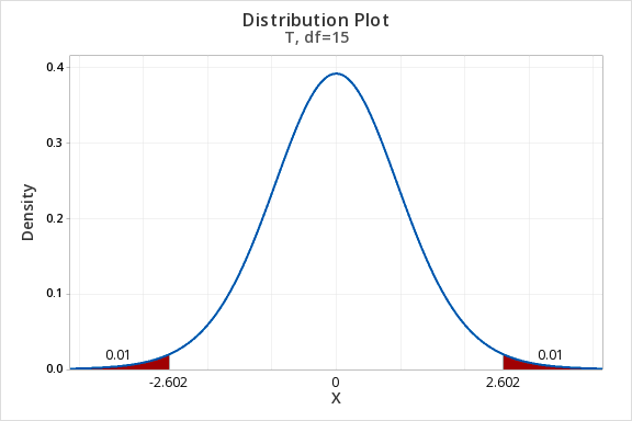
Minitab® – Finding t* Multipliers
To find the t* multiplier for a 98% confidence interval with 15 degrees of freedom:
- In Minitab, select Graph > Probability Distribution Plot > View Probability
- Change the Distribution to t
- Enter 15 for the Degrees of freedom
- Select Options
- Choose A specified probability
- Select Equal tails
- For Probability enter 0.02 (if there is 0.98 in the middle, then 0.02 is split equally between the left and right tails)
This should result in an output similar to the output below. Note that your results may be slightly different due to random sampling variation.
Let’s review some of symbols and equations that we learned in previous lessons:
| Sample size | \(n\) |
|---|---|
| Population mean | \(\mu=\frac{\sum X}{N}\) |
| Sample mean | \(\overline{x}= \frac{\sum x}{n}\) |
| Standard error of the mean | \(SE=\frac{s}{\sqrt{n}}\) |
| Multiplier | \(t^{*} \) |
| Degrees of freedom (one group) | \(df=n-1\) |
Recall the general form for a confidence interval:
- General Form of Confidence Interval
- \(sample\ statistic\pm\underbrace{(multiplier)\ (standard\ error)}_{\textbf{margin of error}}\)
When constructing a confidence interval for a population mean the point estimate is the sample mean, \(\overline{x}\). The multiplier is taken from a \(t\) distribution. And, the standard error is equal to \(\frac{s}{\sqrt{n}}\).
- Confidence Interval for a Population Mean
- \(\underbrace{\overline{x}}_{\text{sample statistic}} \pm \overbrace{t^{*}}^{\text{multiplier}} \underbrace{ \dfrac{s}{\sqrt{n}}}_{\text{standard error}}\)
On the following pages we will walk through examples of constructing confidence intervals for population means by hand. Then, you will learn how to compute confidence intervals using Minitab.
8.2.2.1.1 - Example: MLB Age
8.2.2.1.1 - Example: MLB AgeIn a sample of 30 current MLB pitchers, the mean age was 28 years with a standard deviation of 4.4 years. Construct a 95% confidence interval to estimate the mean age of all current MLB pitchers.
This is what we know: \(n=30\), \(\overline{x}=28\), and \(s=4.4\).
In order to compute the confidence interval for \(\mu\) we will need the t multiplier and the standard error (\( \frac{s}{\sqrt{n}}\)).
\(df=n-1=30-1=29\)
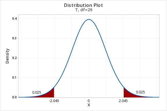
For a 95% confidence interval with 29 degrees of freedom, \(t^{*}=2.045\)
\(SE=\dfrac{s}{\sqrt{n}}=\dfrac{4.4}{\sqrt{30}}=0.803\)
Thus, our confidence interval for \(\mu\) is: \(28\pm 2.045(0.803)=28\pm1.643=[26.357,29.643]\)
We are 95% confident that the population mean age is between 26.357 and 29.643.
8.2.2.1.2- Example: Sleep Deprivation
8.2.2.1.2- Example: Sleep DeprivationIn a class survey, students were asked how many hours they sleep per night. In the sample of 22 students, the mean was 5.77 hours with a standard deviation of 1.572 hours. That distribution was approximately normal. Let’s construct a 95% confidence interval for the mean number of hours slept per night in the population from which this sample was drawn.
This is what we know: \(n=22\), \(\overline{x}=5.77\), and \(s=1.572\).
In order to compute the confidence interval for \(\mu\) we will need the t multiplier and the standard error (\( \frac{s}{\sqrt{n}}\)).
\(df=n-1=22-1=21\)
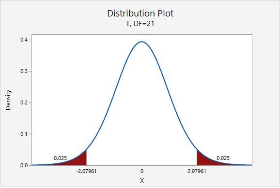
For a 95% confidence interval with 21 degrees of freedom, \(t^{*}=2.080\)
\(SE=\frac{s}{\sqrt{n}}=\frac{1.572}{\sqrt{22}}=0.335\)
Thus, our confidence interval for \(\mu\) is: \(5.77\pm 2.080(0.335)=5.77\pm0.697=[5.073,\;6.467]\)
We are 95% confident that the population mean is between 5.073 and 6.467 hours.
The only thing that would change is our multiplier. Now, \(t^{*}=2.831\).
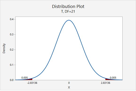
\(5.77\pm 2.831(0.335)=5.77\pm0.948=[4.822,\;6.718]\)
We are 99% confident that the population mean is between 4.822 and 6.718 hours.
8.2.2.1.3 - Example: Milk
8.2.2.1.3 - Example: MilkA study of 66,831 dairy cows found that the mean milk yield was 12.5 kg per milking with a standard deviation of 4.3 kg per milking (data from Berry, et al., 2013). Construct a 95% confidence interval for the average milk yield in the population.
First, let's compute the standard error:
\(SE=\dfrac{s}{\sqrt{n}}=\dfrac{4.3}{\sqrt{66831}}=0.0166\)
The standard error is small because the sample size is very large.
Next, let's find the \(t^*\) multiplier:
\(df=66831-1=66830\)
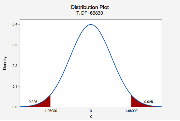
\(t^{*}=1.960\)
Now, we can construct our 95% confidence interval:
95% C.I.: \(12.5\pm1.960(0.017)=12.5\pm0.033=[12.467,\;12.533]\)
We are 95% confident that the mean milk yield in the population is between 12.467 and 12.533 kg per milking.
8.2.2.2 - Minitab: Confidence Interval of a Mean
8.2.2.2 - Minitab: Confidence Interval of a MeanHere you will learn how to use Minitab to construct a confidence interval for a mean. The procedure is similar to the one that you learned earlier in this lesson for constructing a confidence interval for a proportion. The following example walks through this procedure when data are in a Minitab work. At the bottom of this page you will find instructions for using Minitab with summarized data.
Minitab® – Confidence Interval for a Mean
To create a 95% confidence interval of mean height in Minitab:
- Open the data set: fall2016stdata.csv
- In Minitab, select Stat > Basic Statistics > 1-sample t
- In this case we have our data in the Minitab worksheet so we will use the default One or more samples, each in a column
- Double click the variable Height in the box on the left to insert the variable into the box
- Select Options
- The default Confidence level is 95
- Click OK and OK
This should result in the following output:
| N | Mean | StDev | SE Mean | 95% CI for \(\mu\) |
|---|---|---|---|---|
| 525 | 67.009 | 4.462 | 0.195 | (66.627, 67.392) |
\(\mu\): mean of Height
What if we have summarized data and not data in a Minitab worksheet?
If you do not have a Minitab worksheet filled with data concerning individuals, but instead have summarized data (e.g., the values of \(s\), \(\overline{x}\), and \(n\)), you would skip step 1 above and in step 3 you would select Summarized data.
8.2.2.2.1 - Example: Age of Pitchers (Summarized Data)
8.2.2.2.1 - Example: Age of Pitchers (Summarized Data)Example: Estimating the average MLB Pitcher's age
In a sample of 30 current MLB pitchers, the mean age was 28 years with a standard deviation of 4.4 years. Construct a 95% confidence interval to estimate the mean age of all current MLB pitchers.
We know that n = 30, \(\bar{x}=28\), and s = 4.4.
To create a 95% confidence interval of mean age in Minitab:
- In Minitab, select Stat > Basic Statistics > 1-sample t
- In this case we have summarized data so select Summarized Data from the dropdown
- Enter 30 for the sample size, 28 for the sample mean and 4.4 for the standard deviation.
- Select Options
- The default Confidence level is 95
- Click OK and OK
This should result in the following output:
Descriptive Statistics
N | Mean | StDev | SE Mean | 95% CI for \(\mu\) |
|---|---|---|---|---|
30 | 28.000 | 4.400 | 0.803 | (26.357, 29.643) |
\(\mu\): population mean of sample
We are 95% confident that the population mean age is between 26.357 and 29.643 years.
8.2.2.2.2 - Example: Coffee Sales (Data in Column)
8.2.2.2.2 - Example: Coffee Sales (Data in Column)For 48 days data concerning sales were collected from one student-run cafe. Let's construct a 95% confidence interval for the mean number of coffees sold per day.
To create a 95% confidence interval of mean number of coffees sold per day in Minitab:
- Open the file: cafedata.mpx
- In Minitab, select Stat > Basic Statistics > 1-sample t
- In this case the data is in a worksheet so select use One or more samples, each in a column
- Select the variable Coffees
- Select Options
- The default Confidence level is 95
- Click OK and OK
This should result in the following output:
| N | Mean | StDev | SE Mean | 95% CI for \(\mu\) |
|---|---|---|---|---|
| 47 | 21.51 | 11.08 | 1.62 | (18.26, 24.76) |
\(\mu\): population mean of Coffees
We are 95% confident that the population mean number of coffees solder per day is between 18.26 and 24.76.
8.2.2.3 - Computing Necessary Sample Size
8.2.2.3 - Computing Necessary Sample SizeCalculating the sample size necessary for estimating a population mean with a given margin of error and level of confidence is similar to that for estimating a population proportion. However, since the \(t\) distribution is not as “neat” as the standard normal distribution, the process can be iterative. (Recall, the shape of the \(t\) distribution is different for each degree of freedom). This means that we would solve, reset, solve, reset, etc. until we reached a conclusion. Yet, we can avoid this iterative process if we employ an approximate method based on \(t\) distribution approaching the standard normal distribution as the sample size increases. This approximate method invokes the following formula:
- Finding the Sample Size for Estimating a Population Mean
- \(n=\dfrac{z^{2}\widetilde{\sigma}^{2}}{M^{2}}=\left ( \dfrac{z\widetilde{\sigma}}{M} \right )^2\)
-
\(z\) = z multiplier for given confidence level
\(\widetilde{\sigma}\) = estimated population standard deviation
\(M\) = margin of error
The sample standard deviation may be estimated on the basis of prior research studies.
8.2.2.3.1 - Example: Estimating IQ
8.2.2.3.1 - Example: Estimating IQExample: Estimating IQ
A team of researchers wants to estimate the mean IQ of students enrolled at one prestigious university. Previous research studies have examined samples of students from other similar universities and usually find results around \(\overline{x}=120\) and \(s=10\). In order to construct a 90% confidence interval with a margin of error of \(\pm2\) IQ points, what sample size should be obtained?
As shown in the probability distribution plot below, the z value associated with a 90% confidence interval is 1.645.
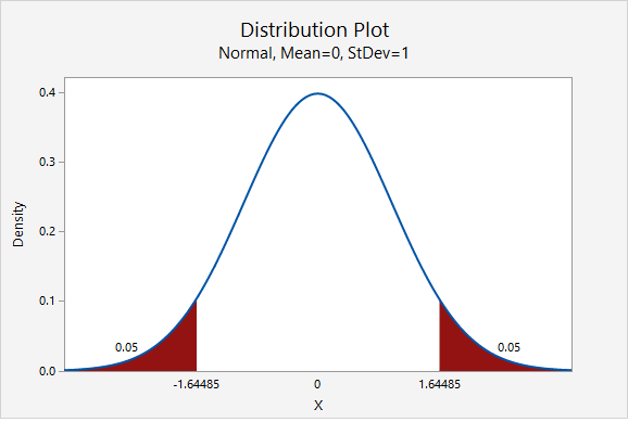
The estimated standard deviation is given to be 10 and the desired margin of error is given to be 2.
\(n=\dfrac{z^{2}\widetilde{\sigma}^{2}}{M^{2}}=\dfrac{1.645^{2}(10^{2})}{2^{2}}=67.615\)
We round up to 68. The research team should attempt to obtain a sample of at least 68 individuals.