8.2.3 - Hypothesis Testing

In this section we will be comparing one sample mean to one known or hypothesized population value. In Lesson 5 you learned how to conduct randomization tests. Here, you will learn how to conduct a one sample mean $t$ test and a one sample mean $z$ test. The $t$ distribution is used to estimate the sampling distribution when the sample size is large (at least 30) or when the population is known to be normally distributed (but $\sigma$ is unknown). The $z$ distribution is used on rare occasions when the population is normal and the population standard deviation is known. Note that for this course the one sample mean $z$ test is optional; it used only in specific cases where the population is known to be normally distributed and when the population standard deviation ($\sigma$) is known. The most commonly used one sample mean test is the "one sample mean $t$ test" which is also known as a "single sample mean $t$ test."

8.2.3.1 - One Sample Mean t Test, Formulas

Five Step Hypothesis Testing Procedure

1. Check assumptions and write hypotheses

Data must be quantitative. In order to use the t distribution to approximate the sampling distribution either the sample size must be large ($\ge\ 30$) or the population must be known to be normally distributed. The possible combinations of null and alternative hypotheses are:

Research Question	Is the mean different from $ \mu_{0} $?	Is the mean greater than $\mu_{0}$?	Is the mean less than $\mu_{0}$?
Null Hypothesis, $H_{0}$	$\mu=\mu_{0} $	$\mu=\mu_{0} $	$\mu=\mu_{0} $
Alternative Hypothesis, $H_{a}$	$\mu\neq \mu_{0} $	$\mu> \mu_{0} $	$\mu<\mu_{0} $
Type of Hypothesis Test	Two-tailed, non-directional	Right-tailed, directional	Left-tailed, directional

where $ \mu_{0} $ is the hypothesized population mean.

2. Calculate the test statistic

For the test of one group mean we will be using a $t$ test statistic:

Test Statistic: One Group Mean

$t=\dfrac{\overline{x}-\mu_0}{\frac{s}{\sqrt{n}}}$

$\overline{x}$ = sample mean
$\mu_{0}$ = hypothesized population mean
$s$ = sample standard deviation
$n$ = sample size

Note that structure of this formula is similar to the general formula for a test statistic:

$\dfrac{sample\;statistic-null\;value}{standard\;error}$

3. Determine the p-value

When testing hypotheses about a mean or mean difference, a $t$ distribution is used to find the $p$-value. These $t$ distributions are indexed by a quantity called degrees of freedom, calculated as $df = n – 1$ for the situation involving a test of one mean or test of mean difference. The $p$-value can be found using Minitab.

4. Make a decision

If $p \leq \alpha$ reject the null hypothesis.

If $p>\alpha$ fail to reject the null hypothesis.

5. State a "real world" conclusion

Based on your decision in Step 4, write a conclusion in terms of the original research question.

The new few pages will walk you through examples before giving you the opportunity to do two on your own.

8.2.3.1.1 - Video Example: Book Costs

Research question: Does the average Penn State student spend more than \$300 each semester on textbooks?

In a sample of 226 Penn State students, the mean cost of a student’s textbooks was \$344 with a standard deviation of \$106.

8.2.3.1.2 : Example: Pulse Rate

A research study measured the pulse rates of 57 college men and found a mean pulse rate of 70.4211 beats per minute with a standard deviation of 9.9480 beats per minute. Researchers want to know if the mean pulse rate for all college men is different from the current standard of 72 beats per minute.

1. Check assumptions and write hypotheses

Pulse rates are quantitative. The sampling distribution will be approximately normally distributed because $n \ge 30$.

This is a two-tailed test because we want to know if the mean pulse rate is different from 72.

$H_{0}:\mu=72 $
$H_{a}: \mu\neq 72 $

2. Calculate the test statistic

Test Statistic: One Group Mean

$t=\dfrac{\overline{x}-\mu_0}{\dfrac{s}{\sqrt{n}}}$

$\overline{x}$ = sample mean
$\mu_{0}$ = hypothesized population mean
$s$ = sample standard deviation
$n$ = sample size

$t=\dfrac{\overline{x}-\mu_0}{\dfrac{s}{\sqrt{n}}}=\dfrac{70.4211-72}{\dfrac{9.9480}{\sqrt{57}}}=-1.198$

Our $t$ test statistic is -1.198

3. Determine the p-value

$df=n-1=57-1=56$

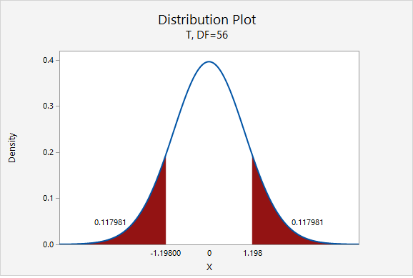
Distribution Plot of Density vs X - T, DF=56

$p=0.117981+0.117981=0.235962$

Given that the null hypothesis is true and $\mu=72$, the probability of taking a random sample of $n=57$ and finding a sample mean this or more extremely different is 0.235962. This is our p-value.

4. Make a decision

$p>.05$, therefore we fail to reject the null hypothesis.

5. State a "real world" conclusion

There is not sufficient evidence to state that the mean pulse of college men is different from 72.

8.2.3.1.3 - Example: Coffee

In the population of Americans who drink coffee, the average daily consumption is 3 cups per day. A university wants to know if their students tend to drink more coffee than the national average. They ask a random sample of 50 students how many cups of coffee they drink each day and found $\overline{x}=3.8$ and $s=1.5$. Do they have evidence that their students drink more than the national average?

1. Check assumption and write hypotheses

Amount of coffee consumed is a quantitative variable. We are given that random sampling methods were employed. Because $n \ge 30$, we can approximate the sampling distribution using a t distribution.

This is a right-tailed test because we want to know if the mean in the sample is greater than the national average.

$H_{0}:\mu= 3$
$H_{a}:\mu>3$

2. Calculate the test statistic

Test Statistic: One Group Mean

$t=\dfrac{\overline{x}-\mu_0}{\dfrac{s}{\sqrt{n}}}$

$\overline{x}$ = sample mean
$\mu_{0}$ = hypothesized population mean
$s$ = sample standard deviation
$n$ = sample size

$t=\dfrac{\overline{x}-\mu_0}{\dfrac{s}{\sqrt{n}}}=\dfrac{3.8-3}{\dfrac{1.5}{\sqrt{50}}}=3.771$

Our $t$ test statistic is 3.771

3. Determine the p-value

$df=n-1=50-1=49$

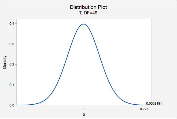
Distribution Plot of Density vs X - T, DF=49

Using Minitab, we can find that $P(t > 3.771) =0.0002191$

p-value = 0.0002191

If $\mu=3$, then the probability of taking a random sample of $n=50$ and finding $\overline{x} \geq 3$ is 0.0002191

4. Make a decision

$p\leq.05$, therefore we reject the null hypothesis.

5. State a "real world" conclusion

There is evidence to state the mean number of coffees consumed in the population of all students at this university is greater than 3.

8.2.3.1.4 - Example: Transportation Costs

According to CNN, in 2011, the average American spent \$16,803 on housing. A suburban community wants to know if their residents spent less than this national average. In a survey of 30 randomly selected residents, they found that they spent an annual average of \$15,800 with a standard deviation of \$2,600.

1. Check assumptions and write hypotheses

Housing costs are quantitative. Because $n \ge 30$, the sampling distribution can be approximated using the $t$ distribution.

This is a left-tailed test because we want to know if residents of this community spent less than the national average.

$H_{0}:\mu=16803$
$H_{a}:\mu<16803$

2. Calculate the test statistic

Test Statistic: One Group Mean

$t=\dfrac{\overline{x}-\mu_0}{\dfrac{s}{\sqrt{n}}}$

$\overline{x}$ = sample mean
$\mu_{0}$ = hypothesized population mean
$s$ = sample standard deviation
$n$ = sample size

$t=\dfrac{\overline{x}-\mu_0}{\dfrac{s}{\sqrt{n}}}=\dfrac{15800-16803}{\dfrac{2600}{\sqrt{30}}}=-2.113$

Our t test statistics is -2.113

3. Determine the p-value

$df=n-1=30-1=29$

This is a left-tailed test so we want to know the probability of $t < -2.113$

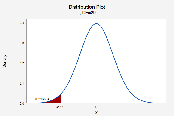
Distribution Plot of Density vs X - T, DF=29

Using Minitab we can find that $p=0.0216634$

4. Make a decision

$p\leq .05$, therefore we reject the null hypothesis.

5. State a "real world" conclusion

There is evidence to state that on average residents of this community spent less than the national average on housing in 2011.

8.2.3.2 - Minitab: One Sample Mean t Tests

A hypothesis test for one group mean can be conducted in Minitab using raw data or summarized data.

If you have a data file with every individual's observation, then you have raw data.
If you do not have each individual's observation, but rather have the sample mean, sample standard deviation, and sample size, then you have summarized data.

The next two pages will show you how to use Minitab to conduct a one-sample mean t-test using either raw data or summarized data. There is also one example of using Minitab to conduct a one-sample mean z test which is only performed if the population is known to be normally distributed and the population standard deviation ($\sigma$) is available.

8.2.3.2.1 - Minitab: 1 Sample Mean t Test, Raw Data

Minitab^® – One Sample Mean t Test Using Raw Data

Research question: Is the mean GPA in the population different from 3.0?

Null hypothesis: $\mu$ = 3.0
Alternative hypothesis: $\mu$ ≠ 3.0

The GPAs of 226 students are available.

A one sample mean $t$ test should be performed because the shape of the population is unknown, however the sample size is large ($n$ ≥ 30).

To perform a one sample mean $t$ test in Minitab using raw data:

Open the Minitab file: class_survey.mpx
Select Stat > Basic Statistics > 1-sample t
Select One or more samples, each in a column from the dropdown
Double-click on the variable GPA to insert it into the Sample box
Check the box Perform a hypothesis test
For the Hypothesized mean enter 3
Select Options
Use the default Alternative hypothesis of Mean ≠ hypothesized value
Use the default Confidence level of 95
Click OK and OK

This should result in the following output:

N	Mean	StDev	SE Mean	95% CI for $\mu$
226	3.2311	0.5104	0.0340	(3.1642, 3.2980)

$\mu$: population mean of GPA

Test
Null hypothesis	H₀: $\mu$ = 3
Alternative hypothesis	H₁: $\mu$ ≠ 3

T-Value	P-Value
6.81	0.000

Summary of Results

We could summarize these results using the five step hypothesis testing procedure:

1. Check assumptions and write hypotheses

We do not know if the population is normally distributed, however the sample size is large ($n \ge 30$) so we can perform a one sample mean t test.

$H_0\colon \mu = 3.0$
$H_a\colon \mu \ne 3.0$

2. Calculate the test statistic

$t (225) = 6.81$

3. Determine the p-value

$p < 0.0001$

4. Make a decision

$p \le \alpha$, reject the null hypothesis

5. State a "real world" conclusion

There is evidence that the mean GPA in the population is different from 3.0

8.2.3.2.2 - Minitab: 1 Sample Mean t Test, Summarized Data

Minitab^® – One Sample Mean t Test Using Summarized Data

Here we are testing $H_{a}\colon\mu\neq72$ and are given $n=35$, $\bar{x}=76.8$, and $s=11.62$.

We do not know the shape of the population, however the sample size is large ($n \ge 30$) therefore we can conduct a one sample mean $t$ test.

To perform a one sample mean $t$ test in Minitab using raw data:

In Minitab, select Stat > Basic Statistics > 1-sample t
Select Summarized data from the dropdown
Enter 35 for the sample size, 76.8 for the sample mean and 11.62 for the standard deviation.
Check the box Perform a hypothesis test
For the Hypothesized mean enter 72
Select Options
Use the default Alternative hypothesis of Mean ≠ hypothesized value
Use the default Confidence level of 95
Click OK and OK

This should result in the following output:

Descriptive Statistics

N	Mean	StDev	SE Mean	95% CI for $\mu$
35	76.80	11.62	1.96	(72.81, 80.79)

$\mu$: population mean of Sample

Test
Null hypothesis	H₀: $\mu$ = 72
Alternative hypothesis	H₁: $\mu$ ≠ 72

T-Value	P-Value
2.44	0.0199

We could summarize these results using the five step hypothesis testing procedure:

1. Check assumptions and write hypotheses

The shape of the population distribution is unknown, however with $n \ge 30$ we can perform a one sample mean t test.

$H_0\colon \mu = 72$
$H_a\colon \mu \ne 72$

2. Calculate the test statistic

$t (34) = 2.44$

3. Determine the p-value

$p = 0.0199$

4. Make a decision

$p \le \alpha$, reject the null hypothesis

5. State a "real world" conclusion

There is evidence that the population mean is different from 72.

8.2.3.3 - One Sample Mean z Test (Optional)

A one sample mean $z$ test is used when the population is known to be normally distributed and when the population standard deviation ($\sigma$) is known. This most frequently occurs in the social sciences when standardized measures are used such as IQ, SAT, ACT, or GRE scores, for which the population parameters are known.

The formula for computing a $z$ test statistic for one sample mean is identical to that of computing a $t$ test statistic for one sample mean, except now the population standard deviation is known and can be used in computing the standard error.

z Test Statistic: One Group Mean: $z=\dfrac{\overline{x}-\mu_0}{\dfrac{\sigma}{\sqrt{n}}}$; $\overline{x}$ = sample mean
$\mu_{0}$ = hypothesized population mean
$s$ = sample standard deviation
$n$ = sample size

The other primary difference between the one sample mean $t$ test and the one sample mean $z$ test is the latter uses the standard normal distribution (i.e., $z$ distribution) in determining the $p$-value. Below are the directions for conducting a one sample mean $z$ test in Minitab.

Minitab^® – Performing a One Sample Mean z Test

Research question: Are the IQ scores of students at one college-prep school above the national average?

Scores on one American IQ test are normed to have a mean of 100 and standard deviation of 15. In a simple random sample of 25 students at this school the mean was 110.

To perform a one-sample mean z test in Minitab using summarized data:

In Minitab, select Stat > Basic Statistics > 1-sample Z
Select Summarized data from the dropdown
Enter 25 for the sample size, 110 for the sample mean and 15 for the known standard deviation.
Check the box Perform a hypothesis test
For the Hypothesized mean enter 100
Select Options
Use the default Alternative hypothesis of Mean > hypothesized value
Use the default Confidence level of 95
Click OK and OK

This should result in the following output:

Descriptive Statistics

N	Mean	SE Mean	95% Lower Bound for $\mu$
25	110.00	3.00	105.07

$\mu$: population mean of Sample
Known standard deviation = 15

Test

Null hypothesis	H₀: $\mu$ = 100
Alternative hypothesis	H₁: $\mu$ > 100

Z-Value	P-Value
3.33	0.000

Summary of Results

We could summarize these results using the five step hypothesis testing procedure:

1. Check assumptions and write hypotheses

The population is known to be normally distributed and the population standard deviation is known to be 15. With these two conditions met we can conduct a one sample mean z test

$H_0\colon \mu = 100$
$H_a\colon \mu > 100$

2. Calculate the test statistic

From the Minitab output, $z = 3.33$

3. Determine the p-value

From the Minitab output, $p = 0.000$

4. Make a decision

$p \le \alpha$, reject the null hypothesis

5. State a "real world" conclusion

There is evidence that the mean IQ score of all students at this school is greater than 100.

Research Question	Is the mean different from \( \mu_{0} \)?	Is the mean greater than \(\mu_{0}\)?	Is the mean less than \(\mu_{0}\)?
Null Hypothesis, \(H_{0}\)	\(\mu=\mu_{0} \)	\(\mu=\mu_{0} \)	\(\mu=\mu_{0} \)
Alternative Hypothesis, \(H_{a}\)	\(\mu\neq \mu_{0} \)	\(\mu> \mu_{0} \)	\(\mu<\mu_{0} \)
Type of Hypothesis Test	Two-tailed, non-directional	Right-tailed, directional	Left-tailed, directional

^[1]	Link
↥	Has Tooltip/Popover
	Toggleable Visibility

Null hypothesis	H₀: \(\mu\) = 3
Alternative hypothesis	H₁: \(\mu\) ≠ 3

Null hypothesis	H₀: \(\mu\) = 72
Alternative hypothesis	H₁: \(\mu\) ≠ 72

Null hypothesis	H₀: \(\mu\) = 100
Alternative hypothesis	H₁: \(\mu\) > 100

8.2.3 - Hypothesis Testing

8.2.3.1 - One Sample Mean t Test, Formulas

Five Step Hypothesis Testing Procedure

8.2.3.1.1 - Video Example: Book Costs

8.2.3.1.2 : Example: Pulse Rate

8.2.3.1.3 - Example: Coffee

8.2.3.1.4 - Example: Transportation Costs

8.2.3.2 - Minitab: One Sample Mean t Tests

8.2.3.2.1 - Minitab: 1 Sample Mean t Test, Raw Data

Minitab® – One Sample Mean t Test Using Raw Data

Summary of Results

8.2.3.2.2 - Minitab: 1 Sample Mean t Test, Summarized Data

Minitab® – One Sample Mean t Test Using Summarized Data

Descriptive Statistics

8.2.3.3 - One Sample Mean z Test (Optional)

Minitab® – Performing a One Sample Mean z Test

Descriptive Statistics

Test

Summary of Results

Minitab^® – One Sample Mean t Test Using Raw Data

Minitab^® – One Sample Mean t Test Using Summarized Data

Minitab^® – Performing a One Sample Mean z Test