8.3 - Paired Means
8.3 - Paired MeansIn Lesson 1 we learned about independent samples and paired samples. When we have two independent samples, the observations in the two groups are unrelated to one another and are not matched in any meaningful way. We'll learn how to compare the means of two independent groups in Lesson 9.
With paired samples, the observations in the two groups are matched in a meaningful way. These are also known as dependent samples. Most often this occurs when data are collected twice from the same participants, called repeated measures. For example, think of studying the effectiveness of a diet plan. You would weigh each participant prior to starting the diet and again following some time on the diet. Depending on how much weight they lost you would determine if the diet was effective. Paired data does not always need to involve two measurements on the same subject; it can also involve taking one measurement on each of two related subjects. For example, we may study husband-wife pairs, mother-son pairs, or pairs of twins.
In constructing a dependent samples confidence interval or conducting a dependent samples hypothesis test, the difference score is computed for each individual or pair. From there, the procedures are the same that you used for constructing confidence intervals and hypothesis tests for single sample means. As with one sample mean, if the sample size is at least 30, the sampling distribution for the difference in paired means can be approximated using a \(t\) distribution.
In terms of symbols, the population parameter of interest is the mean difference in the population "\(\mu_d\)." This is estimated using the mean difference in the sample "\(\overline x_d\)."
8.3.1 - Confidence Intervals
8.3.1 - Confidence IntervalsRecall the general form of a confidence interval...
\(sample\ statistic\pm\underbrace{(multiplier)\ (standard\ error)}_{\textbf{margin of error}}\).
The formula for constructing a confidence interval for the difference in paired means is almost identical to the formula for constructing a confidence interval for one mean. Note that the only change is the subscript d which stands for difference.
Confidence Interval for the Difference Between Two Paired Means
\(\underbrace{\overline{x}_d}_{\text{sample statistic}} \pm \overbrace{t^*}^{\text{multiplier}} \underbrace{\left(\dfrac{s_d}{\sqrt{n}}\right)}_{\text{standard error}}\)
\(t^*\) is the multiplier with \(df = n-1\)
8.3.1.1. - Example: Change in Knowledge
8.3.1.1. - Example: Change in KnowledgeAn educational research study is designed so that participants complete a measure of demonstrated knowledge twice. The researcher wants to estimate the change in scores from the first to second administrations (i.e., pre- and post-test). Data are paired by participant. The researcher subtracted pre-test scores from the post test scores and found a mean increase of 6.560 with a standard deviation of 3.867 for \(n=100\). She wants to construct a 95% confidence interval for the mean difference.
First, we'll find the appropriate multiplier.
\(df=n-1=100-1=99\)
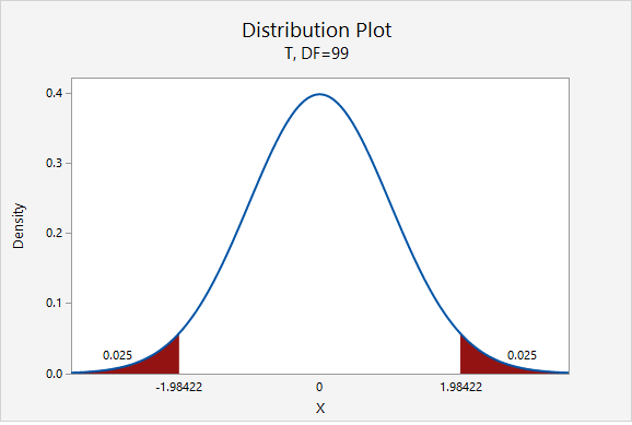
For a 95% confidence interval: \(t_{df=99}=1.984\)
\(6.560 \pm 1.984 \left(\frac{3.867}{\sqrt{100}}\right)=6.560 \pm 0.767=[5.793, 7.327]\)
We are 95% confident that the mean difference between post- and pre- test scores in the population is between 5.793 and 7.327.
Data from Zimmerman, W. A. (2015). Impact of Instructional Materials Eliciting Low and High Cognitive Load on Self-Efficacy and Demonstrated Knowledge (Unpublished doctoral dissertation). The Pennsylvania State University, University Park, PA.
8.3.1.2 - Video Example: Difference in Exam Scores
8.3.1.2 - Video Example: Difference in Exam Scores8.3.2 - Hypothesis Testing
8.3.2 - Hypothesis TestingBelow are the procedures for conducting a hypothesis test for two paired means. This is often referred to as a "paired means \(t\) test," "dependent means \(t\) test," or "matched pairs \(t\) test."
Data must be paired. The difference between the two groups must be normally distributed in the population or the sample size must be at least 30.
The possible combinations of null and alternative hypotheses are:
| Research Question | Is the mean difference different from 0? | Is the mean difference greater than 0? | Is the mean difference less than 0? |
|---|---|---|---|
| Null Hypothesis, \(H_{0}\) | \(\mu_d = 0 \) | \(\mu_d = 0 \) | \(\mu_d = 0 \) |
| Alternative Hypothesis, \(H_{a}\) | \(\mu_d \neq 0 \) | \(\mu_d > 0 \) | \(\mu_d < 0 \) |
| Type of Hypothesis Test | Two-tailed, non-directional | Right-tailed, directional | Left-tailed, directional |
Where \( \mu_d \) is the hypothesized difference in the population.
The calculation of the test statistic for dependent samples is similar to the calculation you performed earlier in this lesson for a single sample mean. In this formula, \(\overline{x}_d\) is used in place of \(\overline{x}\) and \(s_d\) is used in place of \(s\):
- Test Statistic for Dependent Means
-
\(t=\frac{\bar{x}_d-\mu_0}{\dfrac{s_d}{\sqrt{n}}}\)
-
\(\overline{x}_d\) = observed sample mean difference
\(\mu_0\) = mean difference specified in the null hypothesis
\(s_d\) = standard deviation of the differences
\(n\) = sample size (i.e., number of unique individuals)
- Observed Sample Mean Difference
- \(\overline{x}_d=\dfrac{\Sigma{x}_d}{n}\)
- \(x_d\) = observed difference
- Standard Deviation of the Differences
- \(s_d=\sqrt{\dfrac{\sum (x_d-\overline{x}_d)^{2}}{n-1}}\)
When testing hypotheses about a mean difference, a \(t\) distribution is used to find the \(p\) value. The degrees of freedom are equal to \(n-1\) where \(n\) is the number of pairs.
If \(p \leq \alpha\) reject the null hypothesis. If \(p>\alpha\) fail to reject the null hypothesis.
Based on your decision in Step 4, write a conclusion in terms of the original research question.
8.3.2.1 - Example: Quiz Scores
8.3.2.1 - Example: Quiz ScoresBelow is an example of conducting a paired means \(t\) test by hand using raw data. Next, you will learn how this can be conducted most efficiently in Minitab.
Research question: Are scores on two quizzes different?
Data were collected from 9 students and a paired means \(t\) test was performed using hand calculations:
| Student ID | Quiz 1 | Quiz 2 |
|---|---|---|
| 001 | 98 | 94 |
| 002 | 100 | 98 |
| 003 | 95 | 98 |
| 004 | 90 | 88 |
| 005 | 90 | 89 |
| 006 | 92 | 91 |
| 007 | 80 | 84 |
| 008 | 78 | 80 |
| 009 | 88 | 88 |
There are two assumptions: (1) data are paired and (2) distribution of differences is normally distribution in the population or the sample size is at least 30. The data are paired because for each student we have a quiz 1 and a quiz 2 score. We do not know if the differences are normally distributed in the population and the sample size is small, but in the video above we created a histogram of the differences and found that the sample was approximately normally distributed, so this assumption has been met and we can perform a paired means \(t\) test.
Given \(\mu_d = \mu_1 - \mu_2\), our hypotheses are:
\(H_0: \mu_d = 0\)
\(H_a: \mu_d \ne 0\)
- Test Statistic for Dependent Means
-
\(t=\frac{\bar{x}_d-\mu_0}{\frac{s_d}{\sqrt{n}}}\)
\(\overline{x}_d\) = observed sample mean difference
\(\mu_0\) = mean difference specified in the null hypothesis
\(s_d\) = standard deviation of the differences
\(n\) = sample size (i.e., number of unique individuals)
| Student ID | Quiz 1 | Quiz 2 | Difference (\(X_d\)) | \(X_d - \overline{X}_d\) | \((X_d - \overline{X}_d)^2\) |
|---|---|---|---|---|---|
| 001 | 98 | 94 | 4 | 3.889 | 15.123 |
| 002 | 100 | 98 | 2 | 1.889 | 3.568 |
| 003 | 95 | 98 | -3 | -3.111 | 9.679 |
| 004 | 90 | 88 | 2 | 1.889 | 3.568 |
| 005 | 90 | 89 | 1 | 0.889 | 0.790 |
| 006 | 92 | 91 | 1 | 0.889 | 0.790 |
| 007 | 80 | 84 | -4 | -4.111 | 16.901 |
| 008 | 78 | 80 | -2 | -2.111 | 4.457 |
| 009 | 88 | 88 | 0 | -0.111 | 0.012 |
Mean of the differences: \(\overline{X}_d=\frac{\Sigma{X}_d}{n}=\frac{1}{9}\)
For a review of computing standard deviation, see Lesson 2.
Sum of squares: \(\Sigma (X_d - \overline{X}_d)^2 = 54.889\)
Standard deviation of the differences: \(s_d=\sqrt{\frac{\sum (X_d-\overline{X}_d)^{2}}{n-1}} = \sqrt{\frac{54.889}{9-1}}=2.619\)
Test statistic: \(t=\frac{\overline{X}_d- \mu_0}{\frac{s_d}{\sqrt{n}}}=\frac{\frac{1}{9}}{\frac{2.619}{\sqrt{9}}}=0.127\)
\(df=n-1=9-1=8\)
We can construct a \(t\) distribution with 8 degrees of freedom and determine what proportion of the curve falls beyond a \(t\) score of 0.127. This is a two-tailed test, so we need to take into account both the left and right sides of the curve.
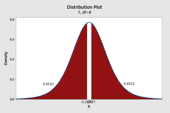
\(p=0.4510+0.4510=0.9020\)
We will compare our \(p\)-value from step 3 to a standard alpha level of 0.05.
Because \(p>\alpha\), we fail to reject the null hypothesis.
There is not sufficient evidence to state that scores on the two quizzes are different.
8.3.3 - Minitab: Paired Means Test
8.3.3 - Minitab: Paired Means TestThe steps for constructing a confidence interval or conducting a paired means \(t\) in Minitab are identical. The output that the procedure provides includes both the confidence interval and the \(p\)-value for determining statistical significance.
Minitab® – Conducting a Paired Means Test
Let's compare students' SAT-Math scores to their SAT-Verbal scores.
- Open the Minitab file: class_survey.mpx
- Select Stat > Basic Statistics > Paired t
- Select Each sample is in a column since we have the data in the worksheet
- Double click the variable SATM in the box on the left to insert the variable into the Sample 1 box
- Double click the variable SATV in the box on the left to insert the variable into the Sample 2 box
- Click OK
This should result in the following output:
Paired t: SATM, SATV
| Sample | N | Mean | StDev | SE Mean |
|---|---|---|---|---|
| SATM | 215 | 599.81 | 84.70 | 5.78 |
| SATV | 215 | 580.33 | 82.44 | 5.62 |
| Mean | StDev | SE Mean | 95% CI for \(\mu_d\) |
|---|---|---|---|
| 19.49 | 89.81 | 6.12 | (7.42, 31.56) |
\(\mu\)_difference: population mean of (SATM - SATV)
| Null hypothesis | H0: \(\mu\)_difference = 0 |
|---|---|
| Alternative hypothesis | H1: \(\mu\)_difference ≠ 0 |
| T-Value | P-Value |
|---|---|
| 3.18 | 0.002 |
On the next page, the five-step hypothesis testing procedure is used to interpret this output.
8.3.3.1 - Example: SAT Scores
8.3.3.1 - Example: SAT ScoresExample: SAT Scores
This example uses the dataset from Lesson 8.3.3 to walk through the five-step hypothesis testing procedure using the Minitab output.
Research question: Do students score differently on the SAT-Math and SAT-Verbal tests?
Because the sample size is large (\(n \ge 30\)), the t distribution may be used to approximate the sampling distribution.
\(H_{0}:\mu_d=0\)
\(H_{a}:\mu_d \ne 0\)
| Null hypothesis | H0: \(\mu_d\) = 0 |
|---|---|
| Alternative hypothesis | H1: \(\mu_d\) ≠ 0 |
| T-Value | P-Value |
|---|---|
| 3.18 | 0.002 |
The t test statistic is 3.18.
From the output, the p value is 0.002
\(p\leq .05\), therefore our decision is to reject the null hypothesis
There is evidence that in the population, on average, students' SAT-Math and their SAT-Verbal scores are different.
8.3.3.2 - Example: Marriage Age (Summarized Data)
8.3.3.2 - Example: Marriage Age (Summarized Data)In a sample of 105 married heterosexual couples, the average age difference (husband's age - wife's age) was 2.829 years with a standard deviation of 4.995 years. These summary statistics were taken from a data set from the Lock5 textbook. Is there convincing evidence that, on average, in the population, husbands tend to be older than their wives?
First we need to check our assumptions. In this case the sample size is greater than 30 so we can use the t-distribution.
We know n = 105, \(\mu_{\text{husband's age}}-\mu_{\text{wife's age}}=2.829\), and \(s=4.995\). Since we want to know if the husbands are older than their wives then our difference in ages would be positive. So our alternative hypothesis is \(H_a\colon \gt 0\).
To complete this using Minitab...
- Select Stat > Basic Statistics > Paired t
- Select Summarized data (differences)
- For sample size enter 105, enter 2.829 for sample mean and 4.995 for standard deviation.
- Select Options
- The Hypothesized difference should be 0. (or 0.0)
- Select Difference > hypothesized difference for the Alternative hypothesis
- Click OK and OK
You should get the following output:
Estimation for Paired Difference
Mean | StDev | SE Mean | 95% CI for \(\mu_d\) |
|---|---|---|---|
105 | 2.829 | 4.995 | (1.862, 3.796 |
\(\mu\)_difference: population mean of (Sample 1 - Sample 2)
Test
Null hypothesis | H0: \(\mu\)_difference = 0 |
|---|---|
Alternative hypothesis | H1: \(\mu\)_difference ≠ 0 |
T-Value | P-Value |
|---|---|
5.80 | 0.000 |
Interpret the results
Because the sample size is large (\(n \ge 30\)), the t distribution may be used to approximate the sampling distribution.
\(H_{0}:\mu_d=0\)
\(H_{a}:\mu_d \gt 0\)
Null hypothesis | H0: \(\mu_d\) = 0 |
|---|---|
Alternative hypothesis | H1: \(\mu_d\) > 0 |
T-Value | P-Value |
|---|---|
5.80 | 0.000 |
The t test statistic is 5.80.
From the output, the p value is 0.000
\(p\leq .05\), therefore our decision is to reject the null hypothesis
There is convincing evidence that in the population, on average, the husband's age in heterosexual couples is greater than the wife's age.