9.1 - Two Independent Proportions
9.1 - Two Independent ProportionsTwo independent proportions tests are used to compare the proportions in two unrelated groups. In StatKey these were known as "Difference in Proportions" tests.
Given that \(n_1 p_1 \ge 10\), \(n_1(1-p_1) \ge 10\), \(n_2 p_2 \ge 10\), and \(n_2(1-p_2) \ge 10\), where the subscript 1 represents the first group and the subscript 2 represents the second group, the sampling distribution will be approximately normal with a standard deviation (i.e., standard error) of \( \sqrt{\frac{p_1(1-p_1)}{n_1}+\frac{p_2(1-p_2)}{n_2}}\). Because the population proportions are not known, they are estimated using the sample proportions. This means if there are at least 10 "successes" and at least 10 "failures" in both groups the sampling distribution for the difference in proportions will be approximately normal.
If the assumption above is met, the normal approximation method is typically preferred. The normal approximation method uses the z distribution to approximate the sampling distribution, similar to the procedures we used in Lesson 7.
When this assumption is not met, Fisher's exact method, bootstrapping, or randomization methods may be used. Fisher's exact method will not be covered in this course. Bootstrapping and randomization methods were covered in Lessons 4 and 5, respectively.
9.1.1 - Confidence Intervals
9.1.1 - Confidence IntervalsGiven that \(np \ge 10\) and \(n(1-p) \ge 10\) for both groups, in other words at least 10 "successes" and at least 10 "failures" in each group, the sampling distribution can be approximated using the normal distribution with a mean of \(\widehat p_1 - \widehat p_2\) and a standard error of \(\sqrt{\frac{p_1(1-p_1)}{n_1}+\frac{p_2(1-p_2)}{n_2}}\).
Recall from the general form of a confidence interval:
- General Form of a Confidence Interval
- \(sample\ statistic\pm(multiplier)\ (standard\ error)\)
Here, the sample statistic is the difference between the two proportions (\(\widehat p_1 - \widehat p_2\)) and the standard error is computed using the formula \(\sqrt{\frac{p_1(1-p_1)}{n_1}+\frac{p_2(1-p_2)}{n_2}}\). Putting this information together, we can derive the formula for a confidence interval for the difference between two proportions.
- Confidence Interval for the Difference Between Two Proportions
- \((\widehat{p}_1-\widehat{p}_2) \pm z^\ast {\sqrt{\dfrac{\widehat{p}_1 (1-\widehat{p}_1)}{n_1}+\dfrac{\widehat{p}_2 (1-\widehat{p}_2)}{n_2}}}\)
Example: Confidence Interval for the Difference Between the Proportion of Women and Men in Favor of Legal Same Sex Marriage
A survey was given to a sample of college students. They were asked whether they think same sex marriage should be legal. Of the 251 women in the sample, 185 said "yes." Of the 199 men in the sample, 107 said "yes." Let’s construct a 95% confidence interval for the difference of the proportion of women and men who responded “yes.” We can apply the 95% Rule and use a multiplier of \(z^\ast\) = 2
- For women: \(np=185\) and \(n(1-p) = 251-185=66\)
- For men: \(np=107\) and \(n(1-p)=199-107=92\)
These counts are all at least 10 so the sampling distribution can be approximated using a normal distribution.
\(\widehat{p}_{w}=\frac{185}{251}=0.737\)
\(\widehat{p}_{m}=\frac{107}{199}=0.538\)
\((0.737-0.538) \pm 2 {\sqrt{\dfrac{0.737 (1-0.737)}{251}+\dfrac{0.538 (1-0.538)}{199}}}\)
\(0.199 \pm 2 ( 0.045)\)
\(.199 \pm .090=[.110, .288]\)
We are 95% confident that in the population the difference between the proportion of women and men who are in favor of same sex marriage legalization is between 0.110 and 0.288.
This confidence interval does not contain 0. Therefore it is not likely that the difference between women and men is 0. We can conclude that there is a difference between the proportion of women and men in the population who would respond “yes" to this question.
9.1.1.1 - Minitab: Confidence Interval for 2 Proportions
9.1.1.1 - Minitab: Confidence Interval for 2 ProportionsMinitab can be used to construct a confidence interval for the difference between two proportions using the normal approximation method. Note that the confidence intervals given in the Minitab output assume that \(np \ge 10\) and \(n(1-p) \ge 10\) for both groups. If this assumption is not true, you should use bootstrapping methods in StatKey.
Minitab® – Constructing a Confidence Interval with Raw Data
Let's estimate the difference between the proportion of females who have tried weed and the proportion of males who have tried weed.
- Open Minitab file: class_survey.mpx
- Select Stat > Basic Statistics > 2 Proportions
- Select Both samples are in one column from the dropdown
- Double click the variable Try Weed in the Samples box
- Double click the variable Biological Sex in the Sample IDs box
- Keep the default Options
- Click OK
This should result in the following output:
Method
Event: Try_Wee = Yes
\(p_1\): proportion where Try_Weed = Yes and Biological Sex = Female
\(p_2\): proportion where Try-Weed = Yes and Biological Sex = Male
Difference: \(p_1\)-\(p_2\)
Descriptive Statistics: Try Weed
| Biological Sex | N | Event | Sample p |
|---|---|---|---|
| Female | 127 | 56 | 0.440945 |
| Male | 99 | 62 | 0.626263 |
Estimation for Difference
| Difference | 95% CI for Difference |
|---|---|
| -0.185318 | (-0.313920, -0.056716) |
CI based on normal approximation
Test
| Null hypothesis | \(H_0\): \(p_1-p_2=0\) |
|---|---|
| Alternative hypothesis | \(H_1\): \(p_1-p_2\neq0\) |
| Method | Z-Value | P-Value |
|---|---|---|
| Normal approximation | -2.82 | 0.005 |
| Fisher's exact | 0.007 |
Minitab® – Constructing a Confidence Interval with Summarized Data
Let's estimate the difference between the proportion of Penn State World Campus graduate students who have children to the proportion of Penn State University Park graduate students who have children. In our representative sample there were 120 World Campus graduate students; 92 had children. There were 160 University Park graduate students; 23 had children.
- Open Minitab
- Select Stat > Basic Statistics > Two-Sample Proportion
- Select Summarized data in the dropdown
- For Sample 1 next to Number of events enter 92 and next to Number of trials enter 120
- For Sample 2 next to Number of events enter 23 and next to Number of trials enter 160
- Keep the default Options
- Click OK
This should result in the following output:
Method
\(p_1\): proportion where Sample 1 = Event
\(p_2\): proportion where Sample 2 = Event
Difference: \(p_1\)-\(p_2\)
Descriptive Statistics
| Sample | N | Event | Sample p |
|---|---|---|---|
| Sample 1 | 120 | 92 | 0.766667 |
| Sample 2 | 160 | 23 | 0.143750 |
Estimation for Difference
| Difference | 95% CI for Difference |
|---|---|
| 0.622917 | (0.529740, 0.716093) |
CI based on normal approximation
| Null hypothesis | \(H_0\): \(p_1-p_2=0\) |
|---|---|
| Alternative hypothesis | \(H_1\): \(p_1-p_2\neq0\) |
| Method | Z-Value | P-Value |
|---|---|---|
| Normal approximation | 13.10 | 0.000 |
| Fisher's exact | 0.000 |
9.1.2 - Hypothesis Testing
9.1.2 - Hypothesis TestingHere we will walk through the five-step hypothesis testing procedure for comparing the proportions from two independent groups. In order to use the normal approximation method there must be at least 10 "successes" and at least 10 "failures" in each group. In other words, \(n p \geq 10\) and \(n (1-p) \geq 10\) for both groups.
If this assumption is not met you should use Fisher's exact method in Minitab or bootstrapping methods in StatKey.
9.1.2.1 - Normal Approximation Method Formulas
9.1.2.1 - Normal Approximation Method Formulas1. Check any necessary assumptions and write null and alternative hypotheses.
To use the normal approximation method a minimum of 10 successes and 10 failures in each group are necessary (i.e., \(n p \geq 10\) and \(n (1-p) \geq 10\)).
The two groups that are being compared must be unpaired and unrelated (i.e., independent).
Below are the possible null and alternative hypothesis pairs:
| Research Question | Are the proportions of group 1 and group 2 different? | Is the proportion of group 1 greater than the proportion of group 2? | Is the proportion of group 1 less than the proportion of group 2? |
|---|---|---|---|
| Null Hypothesis, \(H_{0}\) | \(p_1 - p_2=0\) | \(p_1 - p_2=0\) | \(p_1 - p_2=0\) |
| Alternative Hypothesis, \(H_{a}\) | \(p_1 - p_2 \neq 0\) | \(p_1 - p_2> 0\) | \(p_1 - p_2<0\) |
| Type of Hypothesis Test | Two-tailed, non-directional | Right-tailed, directional | Left-tailed, directional |
The null hypothesis is that there is not a difference between the two proportions (i.e., \(p_1 = p_2\)). If the null hypothesis is true then the population proportions are equal. When computing the standard error for the difference between the two proportions a pooled proportion is used as opposed to the two proportions separately (i.e., unpooled). This pooled estimate will be symbolized by \(\widehat{p}\). This is similar to a weighted mean, but with two proportions.
- Pooled Estimate of \(p\)
- \(\widehat{p}=\dfrac{\widehat{p}_1n_1+\widehat{p}_2n_2}{n_1+n_2}\)
The standard error for the difference between two proportions is symbolized by \(SE_{0}\). The subscript 0 tells us that this standard error is computed under the null hypothesis (\(H_0: p_1-p_2=0\)).
- Standard Error
-
\(SE_0={\sqrt{\dfrac{\widehat{p} (1-\widehat{p})}{n_1}+\dfrac{\widehat{p}(1-\widehat{p})}{n_2}}}=\sqrt{\widehat{p}(1-\widehat{p})\left ( \dfrac{1}{n_1}+\dfrac{1}{n_2} \right )}\)
Note that the default in many statistical programs, including Minitab, is to estimate the two proportions separately (i.e., unpooled). In order to obtain results using the pooled estimate of the proportion you will need to change the method.
Also note that this standard error is different from the one that you used when constructing a confidence interval for \(p_1-p_2\). While the hypothesis testing procedure is based on the null hypothesis that \(p_1-p_2=0\), the confidence interval approach is not based on this premise. The hypothesis testing approach uses the pooled estimate of \(p\) while the confidence interval approach will use an unpooled method.
- Test Statistic for Two Independent Proportions
- \(z=\dfrac{\widehat{p}_1-\widehat{p}_2}{SE_0}\)
The \(z\) test statistic found in Step 2 is used to determine the \(p\) value. The \(p\) value is the proportion of the \(z\) distribution (normal distribution with a mean of 0 and standard deviation of 1) that is more extreme than the test statistic in the direction of the alternative hypothesis.
If \(p \leq \alpha\) reject the null hypothesis. If \(p>\alpha\) fail to reject the null hypothesis.
Based on your decision in Step 4, write a conclusion in terms of the original research question.
9.1.2.1.1 – Example: Ice Cream
9.1.2.1.1 – Example: Ice CreamExample: Ice Cream
The Creamery wants to compare adults and children in terms of preference for eating their ice cream out of a cone. They take a representative sample of 500 customers (240 adults and 260 children) and ask if they prefer cones over bowls. They found that 124 adults preferred cones and 90 children preferred cones.
\(H_0: p_a - p_c = 0\)
\(H_a:p_a - p_c \ne 0\)
Check assumptions:
\(n_a \hat{p}_a = 124\)
\(n_a (1-\widehat p_a) = 240 - 124 = 116\)
\(n_c \widehat p_c = 90\)
\(n_c (1-\widehat p_c) = 260-90 = 170\)
These counts are all at least 10 so we can use the normal approximation method.
Pooled Estimate of \(p\)
\(\widehat{p}=\dfrac{\widehat{p}_1n_1+\widehat{p}_2n_2}{n_1+n_2}\)
\(\widehat{p}=\dfrac{124+90}{240+260}=\dfrac{214}{500}=0.428\)
Standard Error of \(\hat{p}\)
\(SE_{0}={\sqrt{\frac{\widehat{p} (1-\widehat{p})}{n_1}+\frac{\widehat{p}(1-\widehat{p})}{n_2}}}=\sqrt{\widehat{p}(1-\widehat{p})\left ( \frac{1}{n_1}+\frac{1}{n_2} \right )}\)
\(SE_{0}=\sqrt{0.428(1-0.428)\left ( \dfrac{1}{240}+\dfrac{1}{260} \right )}=0.04429\)
Test Statistic for Two Independent Proportions
\(z=\dfrac{\widehat{p}_1-\widehat{p}_2}{SE_0}\)
\(z=\dfrac{\dfrac{124}{240}-\dfrac{90}{260}}{0.04429}=3.850\)
This is a two-tailed test. Our p-value will be the area of the \(z\) distribution more extreme than \(3.850\).
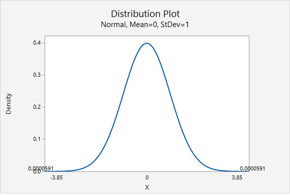
\(p = 0.0000591 \times 2 = 0.0001182\)
\(p \le 0.05\)
Reject the null hypothesis
There is convincing evidence that, in the population of Creamery customers, the proportion of adults who prefer cones is different from the proportion of children who prefer cones in the population.
9.1.2.1.2 – Example: Same Sex Marriage
9.1.2.1.2 – Example: Same Sex MarriageExample: Same Sex Marriage
A survey was given to a random sample of college students. They were asked whether they think same sex marriage should be legal. We're going to compare the students who identified as women and men in terms of whether or not they responded "yes" to this question. Of the 251 women in the sample, 185 said "yes." Of the 199 men in the sample, 107 said "yes."
For women, there were 185 who said "yes" and 66 who said "no." For men, there were 107 who said "yes" and 92 who said "no." There are at least 10 successes and failures in each group so the normal approximation method can be used.
\(\widehat{p}_{w}=\dfrac{185}{251}\)
\(\widehat{p}_{m}=\dfrac{107}{199}\)
This is a two-tailed test because we are looking for a difference between women and men, we were not given a specific direction.
- \( H_{0} : p_{w}- p_{m}=0 \)
- \( H_{a} : p_{w}- p_{m}\neq 0 \)
\(\widehat{p}=\dfrac{185+107}{251+199}=\dfrac{292}{450}=0.6489\)
\(SE_0=\sqrt{\frac{292}{450}\left ( 1-\frac{292}{450} \right )\left ( \frac{1}{251}+\frac{1}{199} \right )}=0.0453\)
\(z=\dfrac{\frac{185}{251}-\frac{107}{199}}{0.0453}=4.400\)
Our test statistic is \(z=4.400\)
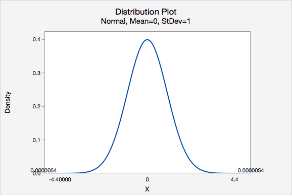
\(P(z>4.400)=0.0000054\), this is a two-tailed test, so this value must be multiplied by two: \(0.0000054\times 2= 0.0000108\)
\(p<0.0001\)
\(p\leq0.05\), therefore we reject the null hypothesis.
There is convincing evidence, in this population of students, that there is a difference between the proportion of women and men who think that same sex marriage should be legal.
9.1.2.2 - Minitab: Difference Between 2 Independent Proportions
9.1.2.2 - Minitab: Difference Between 2 Independent ProportionsWhen conducting a hypothesis test comparing the proportions of two independent proportions in Minitab two p-values are provided. If \(np \ge 10\) and \(n(1-p) \ge 10\), use the p-value associated with the normal approximation method. If this assumption is not met, use the p-value associated with Fisher's exact method.
Minitab Note!
When conducting a hypothesis test for a difference between two independent proportions in Minitab you need to remember to change the "test method" to "use the pooled estimate of the proportion." This is because the null hypothesis is that the two proportions are equal.
Minitab® – Testing Two Independent Proportions using Raw Data
Let's compare the proportion of females who have tried weed to the proportion of males who have tried weed.
- Open Minitab file: class_survey.mpx
- Select Stat > Basic Statistics > 2 Proportions
- Select Both samples are in one column from the dropdown
- Double click the variable Try Weed in the box on the left to insert the variable into the Samples box
- Double click the variable Biological Sex in the box on the left to insert the variable into the Sample IDs box
- Under the Options tab change the Test method to Use the pooled estimate of the proportion
- Click OK and OK
This should result in the following output:
Method
Event: Try_Weed = Yes
\(p_1\): proportion where Try_Weed = Yes and Biological Sex = Female
\(p_2\): proportion where Try-Weed = Yes and Biological Sex = Male
Difference: \(p_1\)-\(p_2\)
Descriptive Statistics: Try Weed
Biological Sex | N | Event | Sample p |
|---|---|---|---|
Female | 127 | 56 | 0.440945 |
Male | 99 | 62 | 0.626263 |
Estimation for Difference
Difference | 95% CI for Difference |
|---|---|
-0.185318 | (-0.313920, -0.056716) |
CI based on normal approximation
Test
Null hypothesis | \(H_0\): \(p_1-p_2=0\) |
|---|---|
Alternative hypothesis | \(H_1\): \(p_1-p_2\neq0\) |
Method | Z-Value | P-Value |
|---|---|---|
Normal approximation | -2.77 | 0.006 |
Fisher's exact | 0.007 |
The test based on the normal approximation uses the pooled estimate of the proportion (0.522124)
Five Step Hypothesis Testing Procedure: Weed Example
Step 1:
\(H_0 : p_f - p_m =0\)
\(H_a : p_f - p_m \neq 0\)
Check assumptions:
\(n_f p_f = 56\)
\(n_f (1-p_f) = 127-56 = 71\)
\(n_m p_m = 62\)
\(n_m (1-p_m) = 99-62 = 37\)
All \(np\) and \(n(1-p)\) are at least ten, therefore we can use the normal approximation method.
Step 2:
From output, \(z=-2.77\)
Step 3:
From output, \(p=0.006\)
Step 4:
\(p \leq \alpha\), reject the null hypothesis
Step 5:
There is convincing evidence that in the population the proportion of females who have tried weed is different from the proportion of males who have tried weed.
Minitab® – Testing Two Independent Proportions using Summarized Data
Let's compare the proportion of Penn State World Campus graduate students who have children to the proportion of Penn State University Park graduate students who have children. In a representative sample there were 120 World Campus graduate students; 92 had children. There were 160 University Park graduate students; 23 had children.
- In Minitab, select Stat > Basic Statistics > 2 Proportions
- Change Both samples are in one column to Summarized data in the dropdown
- For Sample 1 next to Number of events enter 92 and next to Number of trials enter 120
- For Sample 2 next to Number of events enter 23 and next to Number of trials enter 160
- Under the Options tab change the Test method to Use the pooled estimate of the proportion
- Click OK and OK
This should result in the following output:
Method
\(p_1\): proportion where Sample 1 = Event
\(p_2\): proportion where Sample 2 = Event
Difference: \(p_1\)-\(p_2\)
Descriptive Statistics
Sample | N | Event | Sample p |
|---|---|---|---|
Sample 1 | 120 | 92 | 0.766667 |
Sample 2 | 160 | 23 | 0.143750 |
Estimation for Difference
Difference | 95% CI for Difference |
|---|---|
0.622917 | (0.529740, 0.716093) |
CI based on normal approximation
Test
Null hypothesis | \(H_0\): \(p_1-p_2=0\) |
|---|---|
Alternative hypothesis | \(H_1\): \(p_1-p_2\neq0\) |
Method | Z-Value | P-Value |
|---|---|---|
Normal approximation | 10.49 | 0.000 |
Fisher's exact | 0.000 |
The test based on the normal approximation uses the pooled estimate of the proportion (0.410714)
Five Step Hypothesis Testing Procedure: Parents
Step 1:
\(H_0 : p_w - p_u =0\)
\(H_a : p_w - p_u \neq 0\)
Check assumptions:
\(n_w p_w = 92\)
\(n_w (1-p_w) = 120-92 = 28\)
\(n_u p_u = 23\)
\(n_u (1-p_u) = 160-23 = 137\)
All \(np\) and \(n(1-p)\) are at least ten, therefore we can use the normal approximation method.
Step 2:
From output, \(z=10.49\)
Step 3:
From output, \(p=0.000\)
Step 4:
\(p \leq \alpha\), reject the null hypothesis
Step 5:
There is convincing evidence that in the population the proportion of World Campus students who have children is different from the proportion of University Park students who have children.
9.1.2.2.1 - Example: Dating
9.1.2.2.1 - Example: DatingExample: Dating
This example uses the course survey dataset:
A random sample of Penn State University Park undergraduate students were asked, "Would you date someone with a great personality even if you did not find them attractive?" Let's compare the proportion of males and females who responded "yes" to determine if there is convincing evidence of a difference.
We are looking for a "difference," so this is a two-tailed test.
\(H_{0} \colon p_1 - p_2 =0\)
\( H_{a} \colon p_1 - p_2 \neq 0 \)
Check assumptions
\(n_f p_f = 367\)
\(n_f (1-p_f) = 571 - 367 = 204\)
\(n_m p_m = 148\)
\(n_m (1 - p_m) = 433 - 148 = 285\)
All of these counts are at least 10 so we will use the normal approximation method.
From output, \(z=9.45\)
Event: DatePerly = Yes |
\(p_1\): proportion where DatePerly = Yes and Gender = Female |
\(p_2\): proportion where DatePerly = Yes and Gender = Male |
Difference: \(p_1-p_2\) |
Gender | N | Event | Sample p |
|---|---|---|---|
Female | 571 | 367 | 0.642732 |
Male | 433 | 148 | 0.341801 |
Difference | 95% CI for Difference |
|---|---|
0.300931 | (0.241427, 0.360435) |
Null hypothesis | \(H_0\): \(p_1-p_2=0\) |
|---|---|
Alternative hypothesis | \(H_1\): \(p_1-p_2\neq0\) |
Method | Z-Value | P-Value |
|---|---|---|
Fisher's exact | <0.0001 | |
Normal approximation | 9.45 | <0.0001 |
The pooled estimate of the proportion (0.512948) is used for the tests.
From output, \(p<0.0001\)
\(p \leq \alpha\), reject the null hypothesis
There is convincing evidence that in the population of all Penn State University Park undergraduate students the proportion of men who would date someone with a great personality even if they did not find them attractive is different from the proportion of women who would date someone with a great personality even if they did not find them attractive.