9.2.1 - Confidence Intervals
9.2.1 - Confidence IntervalsGiven that the populations are known to be normally distributed, or if both sample sizes are at least 30, then the sampling distribution can be approximated using the \(t\) distribution, and the formulas below may be used. Here you will be introduced to the formulas to construct a confidence interval using the \(t\) distribution. Minitab will do all of these calculations for you, however, it uses a more sophisticated method to compute the degrees of freedom so answers may vary slightly, particularly with smaller sample sizes.
- General Form of a Confidence Interval
- \(point \;estimate \pm (multiplier) (standard \;error)\)
Here, the point estimate is the difference between the two mean, \(\bar{x} _1 - \bar{x}_2\).
- Standard Error
- \(\sqrt{\dfrac{s_1^2}{n_1}+\frac{s_2^2}{n_2}}\)
- Confidence Interval for Two Independent Means
- \((\bar{x}_1-\bar{x}_2) \pm t^\ast{ \sqrt{\frac{s_1^2}{n_1}+\frac{s_2^2}{n_2}}}\)
The degrees of freedom can be approximated as the smallest sample size minus one.
- Estimated Degrees of Freedom
-
\(df=smallest\;n-1\)
Example: Exam Scores by Learner Type
A STAT 200 instructor wants to know how traditional students and adult learners differ in terms of their final exam scores. She collected the following data from a sample of students:
| Traditional Students | Adult Learners | |
|
\(\overline x\) |
41.48 | 40.79 |
| \(s\) | 6.03 | 6.79 |
| \(n\) | 239 | 138 |
She wants to construct a 95% confidence interval to estimate the mean difference.
The point estimate, or "best estimate," is the difference in sample means:
\(\overline x _1 - \overline x_2 = 41.48-40.79=0.69\)
The standard error can be computed next:
\(\sqrt{\dfrac{s_1^2}{n_1}+\dfrac{s_2^2}{n_2}}=\sqrt{\dfrac{6.03^2}{239}+\dfrac{6.79^2}{138}}=0.697\)
To find the multiplier, we need to construct a t distribution with \(df=smaller\;n-1=138-1=137\) to find the t scores that separate the middle 95% of the distribution from the outer 5% of the distribution:
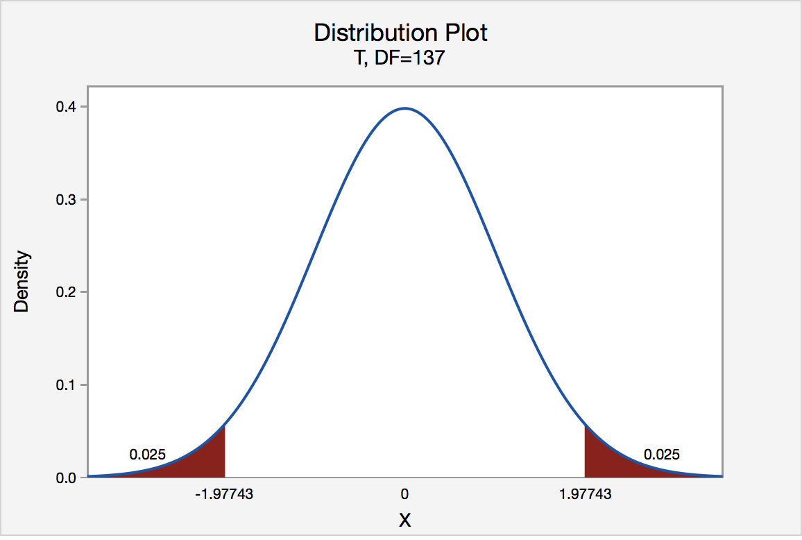
\(t^*=1.97743\)
Now, we can combine all of these values to construct our confidence interval:
\(point \;estimate \pm (multiplier) (standard \;error)\)
\(0.69 \pm 1.97743 (0.697)\)
\(0.69 \pm 1.379\) The margin of error is 1.379
\([-0.689, 2.069]\)
We are 95% confident that the mean difference in traditional students' and adult learners' final exam scores is between -0.689 points and +2.069 points.
9.2.1.1 - Minitab: Confidence Interval Between 2 Independent Means
9.2.1.1 - Minitab: Confidence Interval Between 2 Independent MeansMinitab can be used to construct a confidence interval for the difference between two independent means. Note that the confidence intervals given in the Minitab output assume that either the populations are normally distributed or that both sample sizes are at least 30.
Minitab® – Confidence Interval Between 2 Independent Means
Let's estimate the difference between the mean weight (in pounds) of females and the mean weight of males. Both sample sizes are at least 30 so the sampling distribution can be approximated using the t distribution.
- Open the Minitab file: class_survey.mpx
- Select Stat > Basic Statistics > 2 Sample t
- Select Both samples are in one column from the dropdown
- Double click the variable Weight in the box on the left to insert the variable into the Samples box
- Double click the variable Biological Sex in the box on the left to insert the variable into the Sample IDs box
- Click OK
This should result in the following output:
Method
\(\mu_1\): mean of Weight when Biological Sex = Female
\(\mu_2\): mean of Weight when Biological Sex = Male
Difference: \(\mu_1-\mu_2\)
Equal variances are not assumed for this analysis.
Descriptive Statistics: Weight
| Gender | N | Mean | StDev | SE Mean |
|---|---|---|---|---|
| Female | 126 | 136.7 | 23.4 | 2.1 |
| Male | 99 | 172.7 | 27.3 | 2.7 |
Estimation for Difference
| Difference | 95% CI for Difference |
|---|---|
| -35.99 | (-42.79, -29.20) |
Interpret
I am 95% confident that in the population the mean weight of females is between 29.202 pounds and 42.787 pounds less than the mean weight of males.