11.2.1 - Five Step Hypothesis Testing Procedure
11.2.1 - Five Step Hypothesis Testing ProcedureThe examples on the following pages use the five step hypothesis testing procedure outlined below. This is the same procedure that we used to conduct a hypothesis test for a single mean, single proportion, difference in two means, and difference in two proportions.
When conducting a chi-square goodness-of-fit test, it makes the most sense to write the hypotheses first. The hypotheses will depend on the research question. The null hypothesis will always contain the equalities and the alternative hypothesis will be that at least one population proportion is not as specified in the null.
In order to use the chi-square distribution to approximate the sampling distribution, all expected counts must be at least five.
Expected Count
\(E=np_i\)
Where \(n\) is the total sample size and \(p_i\) is the hypothesized population proportion in the "ith" group.
To check this assumption, compute all expected counts and confirm that each is at least five.
In Step 1 you already computed the expected counts. Use this formula to compute the chi-square test statistic:
Chi-Square Test Statistic
\(\chi^2=\sum \dfrac{(O-E)^2}{E}\)
Where \(O\) is the observed count for each cell and \(E\) is the expected count for each cell.
Construct a chi-square distribution with degrees of freedom equal to the number of groups minus one. The p-value is the area under that distribution to the right of the test statistic that was computed in Step 2. You can find this area by constructing a probability distribution plot in Minitab.
Unless otherwise stated, use the standard 0.05 alpha level.
\(p \leq \alpha\) reject the null hypothesis.
\(p > \alpha\) fail to reject the null hypothesis.
Go back to the original research question and address it directly. If you rejected the null hypothesis, then there is convincing evidence that at least one of the population proportions is not as stated in the null hypothesis. If you failed to reject the null hypothesis, then there is not enough evidence that any of the population proportions are different from what is stated in the null hypothesis.
11.2.1.1 - Video: Cupcakes (Equal Proportions)
11.2.1.1 - Video: Cupcakes (Equal Proportions)11.2.1.2- Cards (Equal Proportions)
11.2.1.2- Cards (Equal Proportions)Example: Cards
Research question: When randomly selecting a card from a deck with replacement, are we equally likely to select a heart, diamond, spade, and club?
I randomly selected a card from a standard deck 40 times with replacement. I pulled 13 hearts, 8 diamonds, 8 spades, and 11 clubs.
Let's use the five-step hypothesis testing procedure:
\(H_0: p_h=p_d=p_s=p_c=0.25\)
\(H_a:\) at least one \(p_i\) is not as specified in the null
We can use the null hypothesis to check the assumption that all expected counts are at least 5.
\(Expected\;count=n (p_i)\)
All \(p_i\) are 0.25. \(40(0.25)=10\), thus this assumption is met and we can approximate the sampling distribution using the chi-square distribution.
\(\chi^2=\sum \dfrac{(Observed-Expected)^2}{Expected} \)
All expected values are 10. Our observed values were 13, 8, 8, and 11.
\(\chi^2=\dfrac{(13-10)^2}{10}+\dfrac{(8-10)^2}{10}+\dfrac{(8-10)^2}{10}+\dfrac{(11-10)^2}{10}\)
\(\chi^2=\dfrac{9}{10}+\dfrac{4}{10}+\dfrac{4}{10}+\dfrac{1}{10}\)
\(\chi^2=1.8\)
Our sampling distribution will be a chi-square distribution.
\(df=k-1=4-1=3\)
We can find the p-value by constructing a chi-square distribution with 3 degrees of freedom to find the area to the right of \(\chi^2=1.8\)
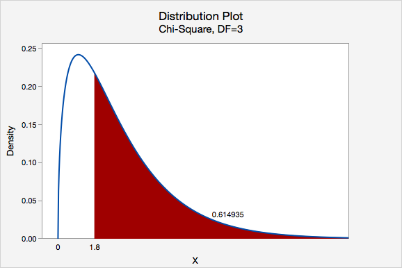
The p-value is 0.614935
\(p>0.05\) therefore we fail to reject the null hypothesis.
There is not enough evidence to state that the proportion of hearts, diamonds, spades, and clubs that are randomly drawn from this deck are different.
11.2.1.3 - Roulette Wheel (Different Proportions)
11.2.1.3 - Roulette Wheel (Different Proportions)Example: Roulette Wheel
Research Question: An American roulette wheel contains 38 slots: 18 red, 18 black, and 2 green. A casino has purchased a new wheel and they want to know if there is convincing evidence that the wheel is unfair. They spin the wheel 100 times and it lands on red 44 times, black 49 times, and green 7 times.
If the wheel is fair then \(p_{red}=\dfrac{18}{38}\), \(p_{black}=\dfrac{18}{38}\), and \(p_{green}=\dfrac{2}{38}\).
All of these proportions combined equal 1.
\(H_0: p_{red}=\dfrac{18}{38},\;p_{black}=\dfrac{18}{38}\;and\;p_{green}=\dfrac{2}{38}\)
\(H_a: At\;least\;one\;p_i\;is \;not\;as\;specified\;in\;the\;null\)
In order to conduct a chi-square goodness of fit test all expected values must be at least 5.
For both red and black: \(Expected \;count=100(\dfrac{18}{38})=47.368\)
For green: \(Expected\;count=100(\dfrac{2}{38})=5.263\)
All expected counts are at least 5 so we can conduct a chi-square goodness of fit test.
\(\chi^2=\sum \dfrac{(Observed-Expected)^2}{Expected} \)
In the first step we computed the expected values for red and black to be 47.368 and for green to be 5.263.
\(\chi^2= \dfrac{(44-47.368)^2}{47.368}+\dfrac{(49-47.368)^2}{47.368}+\dfrac{(7-5.263)^2}{5.263} \)
\(\chi^2=0.239+0.056+0.573=0.868\)
Our sampling distribution will be a chi-square distribution.
\(df=k-1=3-1=2\)
We can find the p-value by constructing a chi-square distribution with 2 degrees of freedom to find the area to the right of \(\chi^2=0.868\)
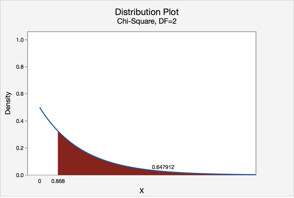
The p-value is 0.647912
\(p>0.05\) therefore we should fail to reject the null hypothesis.
There is not enough evidence that this roulette wheel is unfair.