11.3 - Chi-Square Test of Independence
11.3 - Chi-Square Test of IndependenceThe chi-square (\(\chi^2\)) test of independence is used to test for a relationship between two categorical variables. Recall that if two categorical variables are independent, then \(P(A) = P(A \mid B)\). The chi-square test of independence uses this fact to compute expected values for the cells in a two-way contingency table under the assumption that the two variables are independent (i.e., the null hypothesis is true).
Even if two variables are independent in the population, samples will vary due to random sampling variation. The chi-square test is used to determine if there is convincing evidence that the two variables are not independent in the population using the same hypothesis testing logic that we used with one mean, one proportion, etc.
Again, we will be using the five-step hypothesis testing procedure:
The assumptions are that the sample is randomly drawn from the population and that all expected values are at least 5 (we will see what expected values are later).
Our hypotheses are:
\(H_0:\) There is not a relationship between the two variables in the population (they are independent)
\(H_a:\) There is a relationship between the two variables in the population (they are dependent)
Note: When you're writing the hypotheses for a given scenario, use the names of the variables, not the generic "two variables."
Chi-Square Test Statistic
\(\chi^2=\sum \dfrac{(Observed-Expected)^2}{Expected}\)
Expected Cell Value
\(E=\dfrac{row\;total \; \times \; column\;total}{n}\)
The p-value can be found using Minitab. Look up the area to the right of your chi-square test statistic on a chi-square distribution with the correct degrees of freedom. Chi-square tests are always right-tailed tests.
Degrees of Freedom: Chi-Square Test of Independence
\(df=(number\;of\;rows-1)(number\;of\;columns-1)\)
If \(p \leq \alpha\) reject the null hypothesis.
If \(p>\alpha\) fail to reject the null hypothesis.
Write a conclusion in terms of the original research question.
11.3.1 - Example: Gender and Online Learning
11.3.1 - Example: Gender and Online LearningGender and Online Learning
A sample of 314 Penn State students was asked if they have ever taken an online course. Their genders were also recorded. The contingency table below was constructed. Use a chi-square test of independence to determine if there is a relationship between gender and whether or not someone has taken an online course.
| Have you taken an online course? | ||
|---|---|---|
| Yes | No | |
| Men | 43 | 63 |
| Women | 95 | 113 |
Solution
\(H_0:\) There is not a relationship between gender and whether or not someone has taken an online course (they are independent)
\(H_a:\) There is a relationship between gender and whether or not someone has taken an online course (they are dependent)
Looking ahead to our calculations of the expected values, we can see that all expected values are at least 5. This means that the sampling distribution can be approximated using the \(\chi^2\) distribution.
In order to compute the chi-square test statistic we must know the observed and expected values for each cell. We are given the observed values in the table above. We must compute the expected values. The table below includes the row and column totals.
| Have you taken an online course? | |||
|---|---|---|---|
| Yes | No | ||
| Men | 43 | 63 | 106 |
| Women | 95 | 113 | 208 |
| 138 | 176 | 314 | |
| \(E=\dfrac{row\;total \times column\;total}{n}\) |
| \(E_{Men,\;Yes}=\dfrac{106\times138}{314}=46.586\) |
| \(E_{Men,\;No}=\dfrac{106\times176}{314}=59.414\) |
| \(E_{Women,\;Yes}=\dfrac{208\times138}{314}=91.414\) |
| \(E_{Women,\;No}=\dfrac{208 \times 176}{314}=116.586\) |
Note that all expected values are at least 5, thus this assumption of the \(\chi^2\) test of independence has been met.
Observed and expected counts are often presented together in a contingency table. In the table below, expected values are presented in parentheses.
| Have you taken an online course? | |||
|---|---|---|---|
| Yes | No | ||
| Men | 43 (46.586) | 63 (59.414) | 106 |
| Women | 95 (91.414) | 113 (116.586) | 208 |
| 138 | 176 | 314 | |
\(\chi^2=\sum \dfrac{(O-E)^2}{E} \)
\(\chi^2=\dfrac{(43-46.586)^2}{46.586}+\dfrac{(63-59.414)^2}{59.414}+\dfrac{(95-91.414)^2}{91.414}+\dfrac{(113-116.586)^2}{116.586}=0.276+0.216+0.141+0.110=0.743\)
The chi-square test statistic is 0.743
\(df=(number\;of\;rows-1)(number\;of\;columns-1)=(2-1)(2-1)=1\)
We can determine the p-value by constructing a chi-square distribution plot with 1 degree of freedom and finding the area to the right of 0.743.
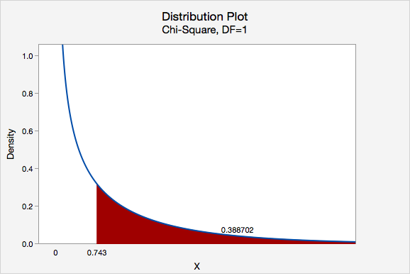
\(p = 0.388702\)
\(p>\alpha\), therefore we fail to reject the null hypothesis.
There is not enough evidence to conclude that gender and whether or not an individual has completed an online course are related.
Note that we cannot say for sure that these two categorical variables are independent, we can only say that we do not have enough evidence that they are dependent.
11.3.2 - Minitab: Test of Independence
11.3.2 - Minitab: Test of IndependenceRaw vs Summarized Data
If you have a data file with the responses for individual cases then you have "raw data" and can follow the directions below. If you have a table filled with data, then you have "summarized data." There is an example of conducting a chi-square test of independence using summarized data on a later page. After data entry the procedure is the same for both data entry methods.
Minitab® – Chi-square Test Using Raw Data
Research question: Is there a relationship between where a student sits in class and whether they have ever cheated?
- Null hypothesis: Seat location and cheating are not related in the population.
- Alternative hypothesis: Seat location and cheating are related in the population.
To perform a chi-square test of independence in Minitab using raw data:
- Open Minitab file: class_survey.mpx
- Select Stat > Tables > Chi-Square Test for Association
- Select Raw data (categorical variables) from the dropdown.
- Choose the variable Seating to insert it into the Rows box
- Choose the variable Ever_Cheat to insert it into the Columns box
- Click the Statistics button and check the boxes Chi-square test for association and Expected cell counts
- Click OK and OK
This should result in the following output:
Rows: Seating Columns: Ever_Cheat
| No | Yes | All | |
|---|---|---|---|
| Back | 24 | 8 | 32 |
| 24.21 | 7.79 | ||
| Front | 38 | 8 | 46 |
| 34.81 | 11.19 | ||
| Middle | 109 | 39 | 148 |
| 111.98 | 36.02 | ||
| All | 1714 | 55 | 226 |
Chi-Square Test
| Chi-Square | DF | P-Value | |
|---|---|---|---|
| Pearson | 1.539 | 2 | 0.463 |
| Likelihood Ratio | 1.626 | 2 | 0.443 |
Interpret
All expected values are at least 5 so we can use the Pearson chi-square test statistic. Our results are \(\chi^2 (2) = 1.539\). \(p = 0.463\). Because our \(p\) value is greater than the standard alpha level of 0.05, we fail to reject the null hypothesis. There is not enough evidence of a relationship in the population between seat location and whether a student has cheated.
11.3.2.1 - Example: Raw Data
11.3.2.1 - Example: Raw DataExample: Dog & Cat Ownership
Is there a relationship between dog and cat ownership in the population of all World Campus STAT 200 students? Let's conduct an hypothesis test using the dataset: fall2016stdata.mpx
\(H_0:\) There is not a relationship between dog ownership and cat ownership in the population of all World Campus STAT 200 students
\(H_a:\) There is a relationship between dog ownership and cat ownership in the population of all World Campus STAT 200 students
Assumption: All expected counts are at least 5. The expected counts here are 176.02, 75.98, 189.98, and 82.02, so this assumption has been met.
Let's use Minitab to calculate the test statistic and p-value.
- After entering the data, select Stat > Tables > Cross Tabulation and Chi-Square
- Enter Dog in the Rows box
- Enter Cat in the Columns box
- Select the Chi-Square button and in the new window check the box for the Chi-square test and Expected cell counts
- Click OK and OK
Rows: Dog Columns: Cat
| No | Yes | All | |
|---|---|---|---|
| No | 183 | 69 | 252 |
| 176.02 | 75.98 | ||
| Yes | 183 | 89 | 272 |
| 189.98 | 82.02 | ||
| Missing | 1 | 0 | |
| All | 366 | 158 | 524 |
Chi-Square Test
| Chi-Square | DF | P-Value | |
|---|---|---|---|
| Pearson | 1.771 | 1 | 0.183 |
| Likelihood Ratio | 1.775 | 1 | 0.183 |
Since the assumption was met in step 1, we can use the Pearson chi-square test statistic.
\(Pearson\;\chi^2 = 1.771\)
\(p = 0.183\)
Our p value is greater than the standard 0.05 alpha level, so we fail to reject the null hypothesis.
There is not enough evidence of a relationship between dog ownership and cat ownership in the population of all World Campus STAT 200 students.
11.3.2.2 - Example: Summarized Data
11.3.2.2 - Example: Summarized DataExample: Coffee and Tea Preference
Is there a relationship between liking tea and liking coffee?
The following table shows data collected from a random sample of 100 adults. Each were asked if they liked coffee (yes or no) and if they liked tea (yes or no).
Likes Coffee | |||
|---|---|---|---|
Yes | No | ||
Likes Tea | Yes | 30 | 25 |
No | 10 | 35 | |
Let's use the 5 step hypothesis testing procedure to address this research question.
\(H_0:\) Liking coffee an liking tea are not related (i.e., independent) in the population
\(H_a:\) Liking coffee and liking tea are related (i.e., dependent) in the population
Assumption: All expected counts are at least 5.
Let's use Minitab to calculate the test statistic and p-value.
Enter the table into a Minitab worksheet as shown below:
C1
C2
C3
Likes Tea
Likes Coffee-Yes
Likes Coffee-No
1
Yes
30
25
2
No
10
35
- Select Stat > Tables > Cross Tabulation and Chi-Square
- Select Summarized data in a two-way table from the dropdown
- Enter the columns Likes Coffee-Yes and Likes Coffee-No in the Columns containing the table box
- For the row labels enter Likes Tea (leave the column labels blank)
- Select the Chi-Square button and check the boxes for Chi-square test and Expected cell counts.
- Click OK and OK
Output
Rows: Likes Tea Columns: Worksheet columns
No | Yes | All | |
|---|---|---|---|
Yes | 30 | 25 | 55 |
22 | 33 | ||
No | 10 | 35 | 45 |
18 | 27 | ||
All | 40 | 60 | 100 |
Chi-Square Test
Chi-Square | DF | P-Value | |
|---|---|---|---|
Pearson | 10.774 | 1 | 0.001 |
Likelihood Ratio | 11.138 | 1 | 0.001 |
Since the assumption was met in step 1, we can use the Pearson chi-square test statistic.
\(Pearson\;\chi^2 = 10.774\)
\(p = 0.001\)
Our p value is less than the standard 0.05 alpha level, so we reject the null hypothesis.
There is convincing evidence of a relationship between between liking coffee and liking tea in the population.
11.3.3 - Relative Risk
11.3.3 - Relative RiskA chi-square test of independence will give you information concerning whether or not a relationship between two categorical variables in the population is likely. As was the case with the single sample and two sample hypothesis tests that you learned earlier this semester, with a large sample size statistical power is high and the probability of rejecting the null hypothesis is high, even if the relationship is relatively weak. In addition to examining statistical significance by looking at the p value, we can also examine practical significance by computing the relative risk.
In Lesson 2 you learned that risk is often used to describe the probability of an event occurring. Risk can also be used to compare the probabilities in two different groups. First, we'll review risk, then you'll be introduced to the concept of relative risk.
The risk of an outcome can be expressed as a fraction or as the percent of a group that experiences the outcome.
- Risk
- \(Risk=\dfrac{n\;with\;outcome}{total\;n}\)
Examples of Risk
Asthma
60 out of 1000 teens have asthma. The risk is \(\frac{60}{1000}=.06\). This means that 6% of all teens experience asthma.
Flu
45 out of 100 children get the flu each year. The risk is \(\frac{45}{100}=.45\) or 45%
- Relative Risk
- Relative risk compares the risk of a particular outcome in two different groups.
- Relative Risk
- \(Relative\ Risk=\dfrac{Risk\ in\ Group\ 1}{Risk\ in\ Group\ 2}\)
Thus, relative risk gives the risk for group 1 as a multiple of the risk for group 2.
Example of Relative Risk
Flu
Suppose that the risk of a child getting the flu this year is .45 and the risk of an adult getting the flu this year is .10. What is the relative risk of children compared to adults?
- \(Relative\;risk=\dfrac{.45}{.10}=4.5\)
Children are 4.5 times more likely than adults to get the flu this year.
Caution
Watch out for relative risk statistics where no baseline information is given about the actual risk. For instance, it doesn't mean much to say that beer drinkers have twice the risk of stomach cancer as non-drinkers unless we know the actual risks. The risk of stomach cancer might actually be very low, even for beer drinkers. For example, 2 in a million is twice the size of 1 in a million but is would still be a very low risk. This is known as the baseline with which other risks are compared.