12.2.1 - Hypothesis Testing
12.2.1 - Hypothesis TestingIn testing the statistical significance of the relationship between two quantitative variables we will use the five step hypothesis testing procedure:
In order to use Pearson's \(r\) both variables must be quantitative and the relationship between \(x\) and \(y\) must be linear
Research Question | Is the correlation in the population different from 0? | Is the correlation in the population positive? | Is the correlation in the population negative? |
|---|---|---|---|
Null Hypothesis, \(H_{0}\) | \(\rho=0\) | \(\rho= 0\) | \(\rho = 0\) |
Alternative Hypothesis, \(H_{a}\) | \(\rho \neq 0\) | \(\rho > 0\) | \(\rho< 0\) |
Type of Hypothesis Test | Two-tailed, non-directional | Right-tailed, directional | Left-tailed, directional |
Minitab will not provide the test statistic for correlation. It will provide the sample statistic, \(r\), along with the p-value (for step 3).
Optional: If you are conducting a test by hand, a \(t\) test statistic is computed in step 2 using the following formula:
\(t=\dfrac{r- \rho_{0}}{\sqrt{\dfrac{1-r^2}{n-2}}} \)
In step 3, a \(t\) distribution with \(df=n-2\) is used to obtain the p-value.
Minitab will give you the p-value for a two-tailed test (i.e., \(H_a: \rho \neq 0\)). If you are conducting a one-tailed test you will need to divide the p-value in the output by 2.
If \(p \leq \alpha\) reject the null hypothesis, there is convincing evidence of a relationship in the population.
If \(p>\alpha\) fail to reject the null hypothesis, there is not enough evidence of a relationship in the population.
Based on your decision in Step 4, write a conclusion in terms of the original research question.
12.2.1.1 - Example: Quiz & Exam Scores
12.2.1.1 - Example: Quiz & Exam ScoresExample: Quiz and exam scores
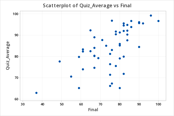
Is there a relationship between students' quiz averages in a course and their final exam scores in the course?
Let's use the 5 step hypothesis testing procedure to address this process research question.
In order to use Pearson's \(r\) both variables must be quantitative and the relationship between \(x\) and \(y\) must be linear. We can use Minitab to create the scatterplot using the file: Exam.mpx
Note that when creating the scatterplot it does not matter what you designate as the x or y axis. We get the following which shows a fairly linear relationship.
Our hypotheses:
- Null Hypothesis, \(H_{0}\): \(\rho=0\)
- Alternative Hypothesis, \(H_{a}\): \(\rho\ne0\)
Use Minitab to compute \(r\) and the p-value.
- Open the file in Minitab
- Select Stat > Basic Statistics > Correlation
- Enter the columns Quiz_Average and Final in the Variables box
- Select the Results button and check the Pairwise correlation table in the new window
- OK and OK
Pairwise Pearson Correlations
| Sample 1 | Sample 2 | N | Correlation | 95% CI for \(\rho\) | P-Value |
|---|---|---|---|---|---|
| Final | Quiz_Average | 50 | 0.609 | (0.398, 0.758) | 0.000 |
Our sample statistic r = 0.609.
From our output the p-value is 0.000.
If \(p \leq \alpha\) reject the null hypothesis, there is evidence of a relationship in the population.
There is evidence of a relationship between students' quiz averages and their final exam scores in the population.
12.2.1.2 - Example: Age & Height
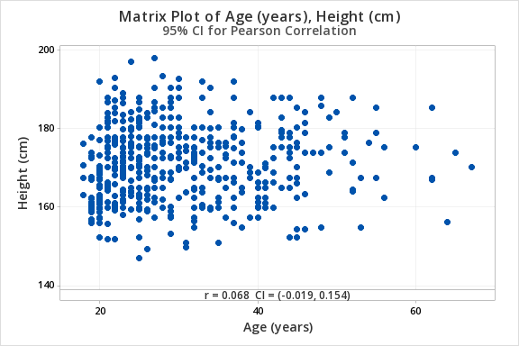
12.2.1.2 - Example: Age & HeightData concerning body measurements from 507 adults retrieved from body.dat.txt for more information see body.txt. In this example, we will use the variables of age (in years) and height (in centimeters) only.
For the full data set and descriptions see the original files:
For this example, you can use the following Minitab file: body.dat.mpx
Research question: Is there a relationship between age and height in adults?
Age (in years) and height (in centimeters) are both quantitative variables. From the scatterplot below we can see that the relationship is linear (or at least not non-linear).
\(H_0: \rho = 0\)
\(H_a: \rho \neq 0\)
From Minitab:
Pairwise Pearson Correlations
| Sample 1 | Sample 2 | N | Correlation | 95% CI for \(\rho\) | P-Value |
|---|---|---|---|---|---|
| Height (cm) | Age (years) | 507 | 0.068 | (-0.019, 0.154) | 0.127 |
\(r=0.068\)
\(p=.127\)
\(p > \alpha\) therefore we fail to reject the null hypothesis.
There is not enough evidence of a relationship between age and height in the population from which this sample was drawn.
12.2.1.3 - Example: Temperature & Coffee Sales
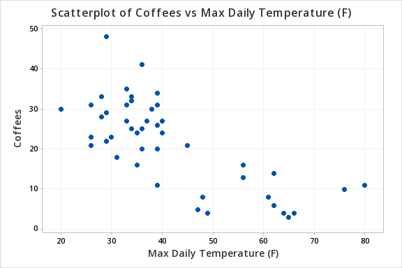
12.2.1.3 - Example: Temperature & Coffee SalesData concerning sales at student-run cafe were retrieved from cafedata.xls more information about this data set available at cafedata.txt. Let's determine if there is a statistically significant relationship between the maximum daily temperature and coffee sales.
For this example, you can use the following Minitab file: cafedata.mpx
Maximum daily temperature and coffee sales are both quantitative variables. From the scatterplot below we can see that the relationship is linear.
\(H_0: \rho = 0\)
\(H_a: \rho \neq 0\)
From Minitab:
Pairwise Pearson Correlations
Sample 1 | Sample 2 | N | Correlation | 95% CI for \(\rho\) | P-Value |
|---|---|---|---|---|---|
Max Daily Temperature (F) | Coffees | 47 | -0.741 | (-0.848, -0.577) | 0.000 |
\(r=-0.741\)
\(p=.000\)
\(p \leq \alpha\) therefore we reject the null hypothesis.
There is convincing evidence of a relationship between the maximum daily temperature and coffee sales in the population.