12.3.4 - Hypothesis Testing for Slope
12.3.4 - Hypothesis Testing for SlopeWe can use statistical inference (i.e., hypothesis testing) to draw conclusions about how the population of \(y\) values relates to the population of \(x\) values, based on the sample of \(x\) and \(y\) values.
The equation \(Y=\beta_0+\beta_1 x\) describes this relationship in the population. Within this model there are two parameters that we use sample data to estimate: the \(y\)-intercept (\(\beta_0\) estimated by \(b_0\)) and the slope (\(\beta_1\) estimated by \(b_1\)). We can use the five step hypothesis testing procedure to test for the statistical significance of each separately. Note, typically we are only interested in testing for the statistical significance of the slope because that tells us that \(\beta_1 \neq 0\) which means that \(x\) can be used to predict \(y\). When \(\beta_1 = 0\) then the line of best fit is a straight horizontal line and having information about \(x\) does not change the predicted value of \(y\); in other words, \(x\) does not help us to predict \(y\). If the value of the slope is anything other than 0, then the predict value of \(y\) will be different for all values of \(x\) and having \(x\) helps us to better predict \(y\).
We are usually not concerned with the statistical significance of the \(y\)-intercept unless there is some theoretical meaning to \(\beta_0 \neq 0\). Below you will see how to test the statistical significance of the slope and how to construct a confidence interval for the slope; the procedures for the \(y\)-intercept would be the same.
The assumptions of simple linear regression are linearity, independence of errors, normality of errors, and equal error variance. You should check all of these assumptions before preceding.
| Research Question | Is the slope in the population different from 0? | Is the slope in the population positive? | Is the slope in the population negative? |
|---|---|---|---|
| Null Hypothesis, \(H_{0}\) | \(\beta_1 =0\) | \(\beta_1= 0\) | \(\beta_1= 0\) |
| Alternative Hypothesis, \(H_{a}\) | \(\beta_1\neq 0\) | \(\beta_1> 0\) | \(\beta_1< 0\) |
| Type of Hypothesis Test | Two-tailed, non-directional | Right-tailed, directional | Left-tailed, directional |
Minitab will compute the \(t\) test statistic:
\(t=\dfrac{b_1}{SE(b_1)}\) where \(SE(b_1)=\sqrt{\dfrac{\dfrac{\sum (e^2)}{n-2}}{\sum (x- \overline{x})^2}}\)
Minitab will compute the p-value for the non-directional hypothesis \(H_a: \beta_1 \neq 0 \)
If you are conducting a one-tailed test you will need to divide the p-value in the Minitab output by 2.
If \(p\leq \alpha\) reject the null hypothesis. If \(p>\alpha\) fail to reject the null hypothesis.
Based on your decision in Step 4, write a conclusion in terms of the original research question.
12.3.4.1 - Example: Quiz and exam scores
12.3.4.1 - Example: Quiz and exam scoresConstruct a model using quiz averages to predict final exam scores.
This example uses the exam data set found in this Minitab file: Exam.mpx
- \(H_0\colon \beta_1 =0\)
- \(H_a\colon \beta_1 \neq 0\)
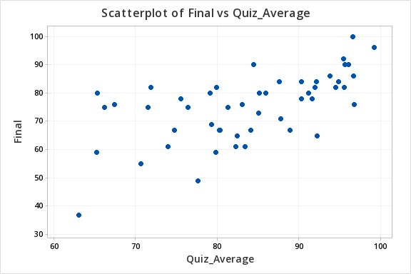
The scatterplot below shows that the relationship between quiz average and final exam score is linear (or at least it's not non-linear).
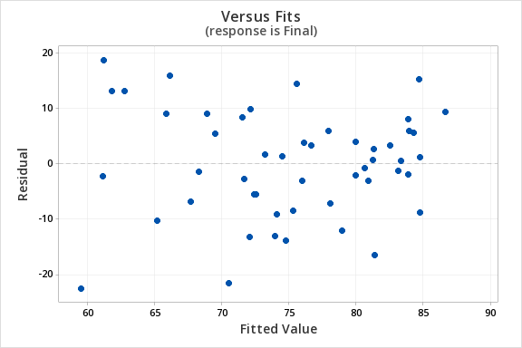
The plot of residuals versus fits below can be used to check the assumptions of independent errors and equal error variances. There is not a significant correlation between the residuals and fits, therefore the assumption of independent errors has been met. The variance of the residuals is relatively consistent for all fitted values, therefore the assumption of equal error variances has been met.
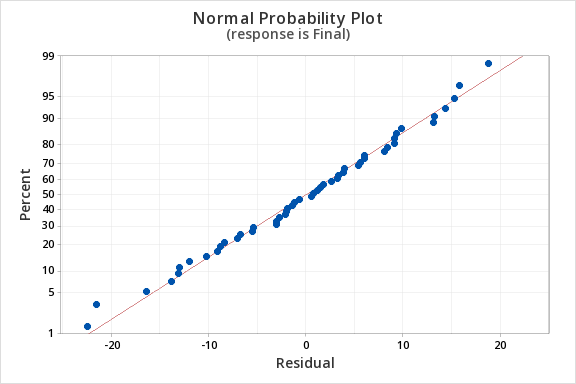
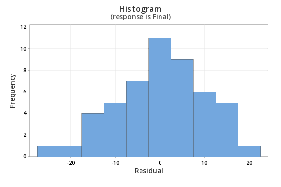
Finally, we must check for the normality of errors. We can use the normal probability plot below to check that our data points fall near the line. Or, we can use the histogram of residuals below to check that the errors are approximately normally distributed.
Now that we have check all of the assumptions of simple linear regression, we can examine the regression model.
We will use the coefficients table from the Minitab output.
Coefficients
Term | Coef | SE Coef | T-Value | P-Value | VIF |
|---|---|---|---|---|---|
Constant | 12.1 | 11.9 | 1.01 | 0.315 | |
Quiz_Average | 0.751 | 0.141 | 5.31 | 0.000 | 1.00 |
\(t = 5.31\)
\(p=0.000\)
\(p < \alpha\), reject the null hypothesis
There is convincing evidence that that students' quiz averages can be used to predict their final exam scores in the population.
12.3.4.2 - Example: Business Decisions
12.3.4.2 - Example: Business DecisionsA student-run cafe wants to use data to determine how many wraps they should make today. If they make too many wraps they will have waste. But, if they don't make enough wraps they will lose out on potential profit. They have been collecting data concerning their daily sales as well as data concerning the daily temperature. They found that there is a statistically significant relationship between daily temperature and coffee sales. So, the students want to know if a similar relationship exists between daily temperature and wrap sales. The video below will walk you through the process of using simple linear regression to determine if the daily temperature can be used to predict wrap sales. The screenshots and annotation below the video will walk you through these steps again.
Can daily temperature be used to predict wrap sales?
Data concerning sales at a student-run cafe were obtained from a Journal of Statistics Education article. Data were retrieved from cafedata.xls more information about this data set available at cafedata.txt.
For the analysis you can use the Minitab file: cafedata.mpx
- \(H_0\colon \beta_1 =0\)
- \(H_a\colon \beta_1 \neq 0\)
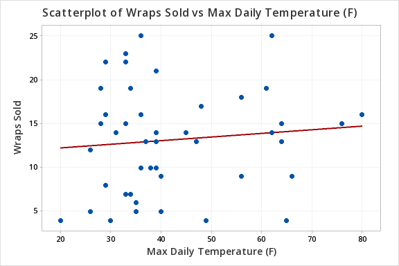
The scatterplot below shows that the relationship between maximum daily temperature and wrap sales is linear (or at least it's not non-linear). Though the relationship appears to be weak.
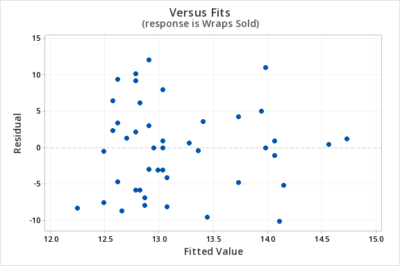
The plot of residuals versus fits below can be used to check the assumptions of independent errors and equal error variances. There is not a significant correlation between the residuals and fits, therefore the assumption of independent errors has been met. The variance of the residuals is relatively consistent for all fitted values, therefore the assumption of equal error variances has been met.
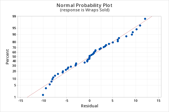
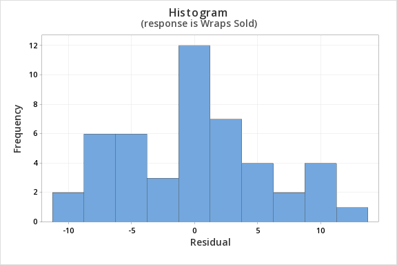
Finally, we must check for the normality of errors. We can use the normal probability plot below to check that our data points fall near the line. Or, we can use the histogram of residuals below to check that the errors are approximately normally distributed.
Now that we have check all of the assumptions of simple linear regression, we can examine the regression model.
Regression Equation
Wraps Sold = 11.42 + 0.0414 Max Daily Temperature (F)
Coefficients
| Term | Coef | SE Coef | T-Value | P-Value | VIF |
|---|---|---|---|---|---|
| Constant | 11.42 | 2.66 | 4.29 | 0.000 | |
| Max Daily Temperature (F) | 0.0414 | 0.0603 | 0.69 | 0.496 | 1.00 |
Model Summary
| S | R-sq | R-sq(adj) | R-sq(pred) |
|---|---|---|---|
| 5.90208 | 1.04% | 0.00% | 0.00% |
Analysis of Variance
| Source | DF | Adj SS | Adj MS | F-Value | P-Value |
|---|---|---|---|---|---|
| Regression | 1 | 16.41 | 16.41 | 0.47 | 0.496 |
| Max Daily Temperature (F) | 1 | 16.41 | 16.41 | 0.47 | 0.496 |
| Error | 45 | 1567.55 | 34.83 | ||
| Lack-of-Fit | 24 | 875.17 | 36.47 | 1.11 | 0.411 |
| Pure Error | 21 | 692.38 | 32.97 | ||
| Total | 46 | 1583.96 |
\(t = 0.69\)
\(p=0.496\)
\(p > \alpha\), fail to reject the null hypothesis
There is not enough evidence to conclude that maximum daily temperature can be used to predict the number of wraps sold in the population of all days.