8.2.1 - t Distribution
8.2.1 - t DistributionThe height of the t distribution is determined by the number of degrees of freedom (df). For a one sample mean test, \(df=n-1\).
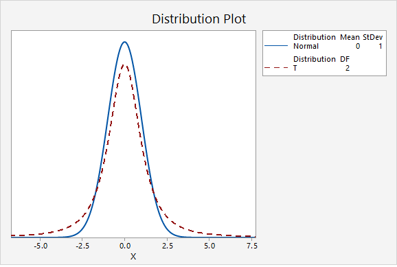
The first plot below compares the standard normal distribution (i.e., z distribution) to a t distribution. The solid blue line is the standard normal distribution and the dashed red line is a t distribution with 2 degrees of freedom. Here, the tails of the t distribution are higher than the tails of the normal distribution.
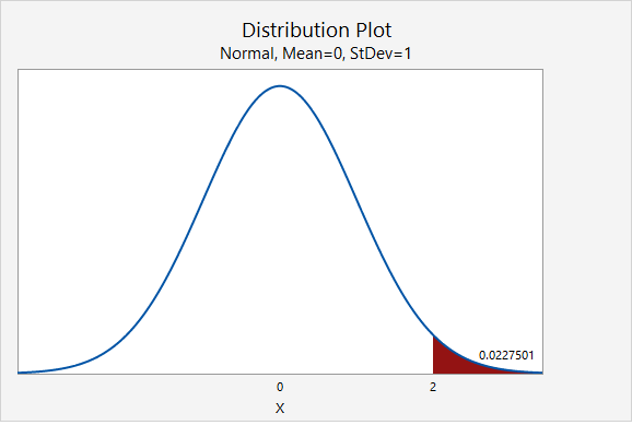
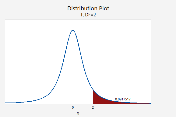
If you think about the area under the curve, the higher tails mean that more area will fall in the tails. For example, as seen in the following two plots, \(P(z>2.00)=0.0227501\) while \(P(t_{df=2}>2.00)=0.0917517\).
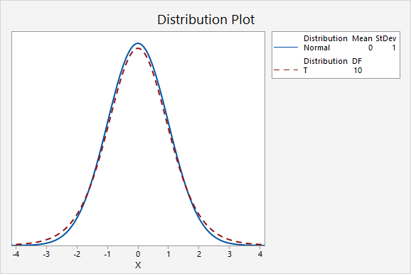
The next plot compares the standard normal distribution to a t distribution with 10 degrees of freedom. Notice that the two distributions are becoming more similar as the sample size increases.
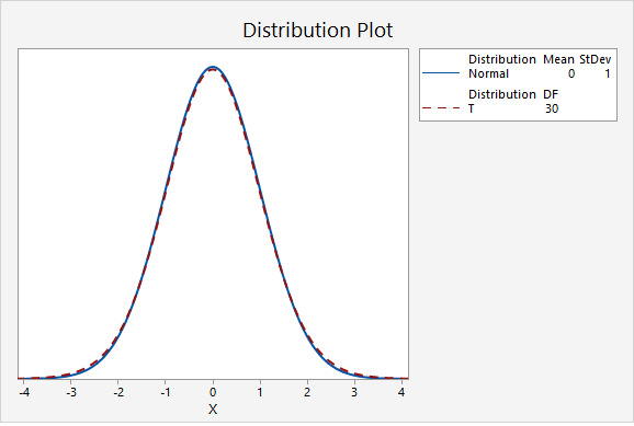
The next plot compares the standard normal distribution to a t distribution with 30 degrees of freedom.
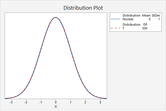
In the final graph, the standard normal distribution is compared to a t distribution with 500 degrees of freedom. Here, the two distributions are nearly identical. As the degrees of freedom approach infinity, the t distribution approaches (i.e., becomes more similar to) the standard normal distribution.
Minitab®
The procedures for constructing t distributions in Minitab are similar to those for constructing z distributions. We can construct a probability distribution plot to find the t* multiplier when constructing a confidence interval. And, we can construct a plot to find the p-value when conducting a hypothesis test.
Steps for finding the t* multiplier
- In Minitab, select Graph > Probability Distribution Plot > View Probability
- Change the Distribution to t
- Enter your Degrees of freedom
- Select Options
- Choose A specified probability
- Select Equal tails
- For Probability enter the value that is split between the two tails (e.g., for a 90% confidence interval you would enter 0.10)
Steps for finding the p value given a t test statistic
- In Minitab, select Graph > Probability Distribution Plot > View Probability
- Change the Distribution to t
- Enter your Degrees of freedom
- Select A specified x value
- Select Right tail, Left tail, or Equal tails, depending on the direction of your alternative hypothesis
- For X value enter the t test statistic