8: Inference for One Sample
8: Inference for One SampleObjectives
- Identify situations in which the z or t distributions may be used to approximate a sampling distribution
- Construct a confidence interval to estimate a population proportion, mean, or difference in paired means by hand given summary data
- Construct a confidence interval to estimate a population proportion, mean, or difference in paired means using Minitab given summary or raw data
- Determine the necessary minimum sample size to construct a confidence interval for a single proportion or single mean with a given level of confidence and margin of error
- Conduct a hypothesis test using the appropriate common distribution for a single proportion, single mean, and paired means by hand given summary data
- Conduct a hypothesis test using the appropriate common distribution for a single proportion, single mean, and paired means using Minitab given summary or raw data
This lesson corresponds to Chapter 6 in the Lock5 textbook.
The general form of confidence intervals and test statistics will be the same for all of the procedures covered in this lesson:
- General Form of a Confidence Interval
- \(sample\ statistic\pm(multiplier)\ (standard\ error)\)
- General Form of a Test Statistic
- \(test\;statistic=\dfrac{sample\;statistic-null\;parameter}{standard\;error}\)
We will be using a five step hypothesis testing procedure:
- Check assumptions and write hypotheses. The assumptions will vary depending on the test. The null and alternative hypotheses will also be written in terms of population parameters; the null hypothesis will always contain the equality (i.e., \(=\)).
- Calculate the test statistic. This will vary depending on the test, but it will typically be the difference observed between the sample and population divided by a standard error. In this lesson, we will see z and t test statistics. Minitab will compute the test statistic.
- Determine the p-value. This can be found using Minitab.
- Make a decision. If \(p \leq \alpha\) reject the null hypothesis. If \(p>\alpha\) fail to reject the null hypothesis.
- State a "real world" conclusion. Based on your decision in step 4, write a conclusion in terms of the original research question.
Some steps may vary depending on the test.
We will be relying heavily on Minitab in this lesson and all of the following lessons. Note that help is available in Minitab.
8.1 - One Sample Proportion
8.1 - One Sample ProportionOne sample proportion tests and confidence intervals are covered in Section 6.1 of the Lock5 textbook.
In the last lesson you were introduced to the general concept of the Central Limit Theorem. The Central Limit Theorem states that if the sample size is sufficiently large then the sampling distribution will be approximately normally distributed for many frequently tested statistics, such as those that we have been working with in this course. When discussion proportions, we sometimes refer to this as the Rule of Sample Proportions. According to the Rule of Sample Proportions, if \(np\geq 10\) and \(n(1-p) \geq 10\) then the sampling distributing will be approximately normal. When constructing a confidence interval \(p\) is not known but may be approximated using \(\widehat p\). When conducting a hypothesis test, we check this assumption using the hypothesized proportion (i.e., the proportion in the null hypothesis).
If assumptions are met, the sampling distribution will have a standard error equal to \(\sqrt{\frac{p(1-p)}{n}}\).
This method of constructing a sampling distribution is known as the normal approximation method.
If the assumptions for the normal approximation method are not met (i.e., if \(np\) or \(n(1-p)\) is not at least 10), then the sampling distribution may be approximated using a binomial distribution. This is known as the exact method. This course does not cover the exact method in detail, but you will see how these tests may be performed using Minitab.
8.1.1 - Confidence Intervals
8.1.1 - Confidence IntervalsOn the following pages you will see how a confidence interval for a population proportion can be constructed by hand using the normal approximation method. Using Minitab, you will learn how to construct a confidence interval for a proportion using the normal approximation method or the exact method. When given the option, it is recommended that you use Minitab as opposed to performing calculations by hand.
8.1.1.1 - Normal Approximation Formulas
8.1.1.1 - Normal Approximation FormulasFor the following procedures, the assumption is that both \(np \geq 10\) and \(n(1-p) \geq 10\). When we're constructing confidence intervals \(p\) is typically unknown, in which case we use \(\widehat{p}\) as an estimate of \(p\).
Note that \(n \widehat p\) is the number of successes in the sample and \(n(1- \widehat p)\) is the number of failures in the sample.
This means that our sample needs to have at least 10 "successes" and at least 10 "failures" in order to construct a confidence interval using the normal approximation method.
Below is the general form of a confidence interval.
- General Form of Confidence Interval
- \(sample\ statistic\pm\underbrace{(multiplier)\ (standard\ error)}_{\textbf{margin of error}}\)
The sample statistic here is the sample proportion, \(\widehat p\). When using the normal approximation method the multiplier is taken from the standard normal distribution (i.e., z distribution). And, the standard error is computed using \(\widehat p\) as an estimate of \(p\): \(\sqrt{\frac{\hat{p} (1-\hat{p})}{n}}\). This leaves us with the following formula to construct a confidence interval for a population proportion:
- Confidence Interval of \(p\): Normal Approximation Method
- \(\underbrace{\widehat{p}}_{\text{sample statistic}} \pm \overbrace{z^{*}}^{\text{multiplier}} \underbrace{\left (\sqrt{\frac{\hat{p}(1-\hat{p})}{n}}\right)}_{\text{standard error}} \)
Finding the z* Multiplier
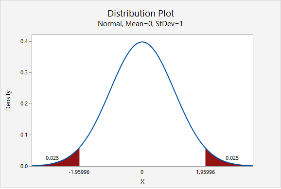
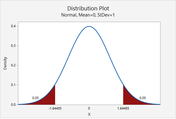
The value of the \(z^*\) multiplier depends on the level of confidence. The multiplier for the confidence interval for a population proportion can be found using the standard normal distribution [i.e., z distribution, N(0,1)]. The most commonly used level of confidence is 95%. As shown on the probability distribution plot below, the multiplier associated with a 95% confidence interval is 1.960, often rounded to 2 (recall the Empirical Rule and 95% Rule).
Below is a table of frequently used \(z^*\) multipliers.
| Confidence Level | \(z^*\) Multiplier |
|---|---|
| 90% | 1.645 |
| 95% | 1.960, often rounded to 2 |
| 98% | 2.327 |
| 99% | 2.576 |
The value of the multiplier increases as the confidence level increases. This leads to wider intervals for higher confidence levels. We are more confident of catching the population value when we use a wider interval.
8.1.1.1.1 - Video Example: PA Residency
8.1.1.1.1 - Video Example: PA Residency8.1.1.1.2 - Video Example: Dog Ownership
8.1.1.1.2 - Video Example: Dog OwnershipIn Spring 2016, a sample of 522 World Campus students were surveyed and asked if they own a dog. Of the 522 students in the sample, 273 said that they did have a dog. Construct a 95% confidence interval for the proportion of all World Campus students who have a dog.
8.1.1.1.3 - Video Example: Books
8.1.1.1.3 - Video Example: Books8.1.1.1.4 - Example: Retirement
8.1.1.1.4 - Example: RetirementIn a representative sample of 1168 American adults, 747 said they were not financially prepared for retirement. Let's construct a 95% confidence interval to estimate the proportion of all American adults who are not financially prepared for retirement.
First, we need to check our assumptions that both \(n\widehat p \geq 10\) and \(n(1-\widehat p) \geq 10\).
\(\widehat{p}=\frac{747}{1168}=0.640\)
\(np=1168 (0.640) = 747\) and \(n(1-p)=1168(1-0.640)=421\)
Both are greater than 10, so this assumption has been met. This means we can use the normal approximation method to construct this confidence interval.
Next, we can compute the standard error.
\(SE=\sqrt{\frac{\hat{p} (1-\hat{p})}{n}}=\sqrt{\frac{0.640 (1-0.640)}{1168}}=0.014\)
The \(z^*\) multiplier for a 95% confidence interval is 1.960
The formula for a confidence interval for a proportion is \(\widehat{p}\pm z^* (SE)\)
\(0.640\pm 1.960(0.014)=0.640\pm0.028=[0.612, \;0.668]\)
We are 95% confident that between 61.2% and 66.8% of all American adults are not financially prepared for retirement.
Let’s think about how our interval will change. The 99% confidence interval will be wider than the 95% confidence interval. In order to increase our level of confidence, we will need to expand the interval.
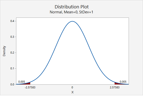
In terms of computing the 99% confidence interval, we will use the same point estimate \(\widehat{p}\) and the same standard error. Only the multiplier will change. From the plot below, we see that the \(z^*\) multiplier for a 99% confidence interval is 2.576.
\(99\%\;C.I.:\;0.640\pm 2.576 (0.014)=0.0640\pm 0.036=[0.604, \; 0.676]\)
We are 99% confidence that between 60.4% and 67.6% of all American adults are not financially prepared for retirement.
8.1.1.2 - Minitab: Confidence Interval for a Proportion
8.1.1.2 - Minitab: Confidence Interval for a ProportionBefore we can construct a confidence interval for a proportion we must first determine if we should use the exact method or the normal approximation method. Recall that if \(np \geq 10\) and \(n(1-p) \geq 10\) then the sampling distribution can be approximated by a normal distribution. Since we don't have the population proportion (\(p\)), we using \(\widehat p\) as an estimate. Note that \(n\widehat p\) is the number of successes in the sample and \(n(1-\widehat p)\) is the number of failures in the sample.
If this assumption has not been met, then the sampling distribution is constructed using a binomial distribution which Minitab refers to as the "exact method."
To check this assumption we can construct a frequency table. You first learned how to construct a frequency table in Lesson 2.1.1.2.1 of these online notes. Here is another example:
Minitab® – Frequency Tables
To create a frequency table of dog ownership in Minitab:
- Open the data set:
- From the toolbar in Minitab, select Stat > Tables > Tally Individual Variables
- Double click the variable Dog in the box on the left to insert the variable into the Variable box
- Under Display, choose Counts
- Click OK
This should result in the following frequency table:
| Dog | Count |
|---|---|
| No | 252 |
| Yes | 272 |
| N= | 524 |
| *= | 1 |
From the frequency table above we can see that there were at least 10 "successes" and at least 10 "failures" in the sample. In this example a success is defined as answering "yes" to the question "do you own a dog?" A failure is defined as answering "no." Because both \(n \widehat p \geq 10\) and \(n(1- \widehat p) \geq 10\), the normal approximation method may be used. In Minitab, the exact method is the default method. If there are at least 10 successes and at least 10 failures, then you need to change the method to the normal approximation method.
Minitab® – Confidence Interval for a Proportion (Normal Approximation)
To create a 95% confidence interval of dog ownership using the normal approximation method in Minitab:
- Open the data set: fall2016stdata.mpx
- In Minitab, select Stat > Basic Statistics > 1-Proportion
- In this case we have our data in the Minitab worksheet so we will use the default One or more samples each in a column.
- Double click the variable Dog in the box on the left to insert the variable into the box.
- Select Options
- The default Confidence level is 95
- Change the Method to Normal approximation because the assumption of \(n \widehat p \geq 10\) and \(n(1- \widehat p) \geq 10\) has been met
- Click OK
This should result in the following output:
Method
Event: Dog = Yes
p: proportion where Dog = Yes
Normal approximation is used for this analysis.
| N | Event | Sample p | 95% CI for p |
|---|---|---|---|
| 524 | 272 | 0.519084 | (0.476304, 0.561863) |
What if the assumption is not met?
If the number of successes or the number of failures in the sample is less than 10, then the exact method should be used instead of the normal approximation method. In Minitab, this means that in step 8 above the default setting of Exact method should not be changed.
If you do not have a Minitab worksheet filled with data concerning individuals, but instead have summarized data (e.g., the number of successes and the number of failures), you would not load the data set, but in step 3 you would select Summarized data. For Number of events, enter the number of successes (i.e., \(n \widehat p\)) and for Number of trials enter the total sample size (i.e., \(n\)).
8.1.1.2.1 - Example with Summarized Data
8.1.1.2.1 - Example with Summarized DataExample: Lactose Intolerance
In a sample of 100 African American adults, 70 were identified as having some level of lactose intolerance. Compute a 95% confidence interval to estimate the proportion of all African American adults who have some level of lactose intolerance.
To create a 95% confidence interval of dog ownership using the normal approximation method in Minitab:
-
- In this case we have summarized data so select Summarized data in the dropdown.
- For number of events, add 70 and for number of trials add 100.
- Select Options
- The default Confidence level is 95.
- Change the Method to Normal approximation because the assumption of \(n \widehat p \geq 10\) and \(n(1- \widehat p) \geq 10\) has been met
- Click OK and OK.
This should result in the following output:
Method
p: event proportion
Normal approximation is used for this analysis.
| N | Event | Sample p | 95% CI for p |
|---|---|---|---|
| 100 | 70 | 0.700000 | (0.610183, 0.789817) |
8.1.1.2.2 - Example with Summarized Data
8.1.1.2.2 - Example with Summarized DataExample: Dieting
At the beginning of the Fall 2016 semester a representative sample of World Campus STAT 200 students was surveyed. The students were asked if they were currently dieting to lose weight. In the sample of 524 students, 184 said that they were dieting to lose weight. Construct a 95% confidence interval for the proportion of all World Campus STAT 200 students who are dieting to lose weight.
-
- In this case we have summarized data so select Summarized data in the dropdown.
- For number of events, add 184 and for number of trials add 524.
- Select Options
- The default Confidence level is 95.
- Change the Method to Normal approximation because the assumption of \(n \widehat p \geq 10\) and \(n(1- \widehat p) \geq 10\) has been met
- Click OK and OK.
This should result in the following output:
Method
p: event proportion
Normal approximation is used for this analysis.
| N | Event | Sample p | 95% CI for p |
|---|---|---|---|
| 524 | 184 | 0.351145 | (0.310276, 0.392015) |
8.1.1.3 - Computing Necessary Sample Size
8.1.1.3 - Computing Necessary Sample SizeWhen we begin a study to estimate a population parameter we typically have an idea as how confident we want to be in our results and within what degree of accuracy. This means we get started with a set level of confidence and margin of error. We can use these pieces to determine a minimum sample size needed to produce these results by using algebra to solve for \(n\):
- Finding Sample Size for Estimating a Population Proportion
- \(n=\left ( \dfrac{z^*}{M} \right )^2 \tilde{p}(1-\tilde{p})\)
-
\(M\) is the margin of error
\(\tilde p\) is an estimated value of the proportion
If we have no preconceived idea of the value of the population proportion, then we use \(\tilde{p}=0.50\) because it is most conservative and it will give use the largest sample size calculation.
Example: No Estimate
We want to construct a 95% confidence interval for \(p\) with a margin of error equal to 4%.
Because there is no estimate of the proportion given, we use \(\tilde{p}=0.50\) for a conservative estimate.
For a 95% confidence interval, \(z^*=1.960\)
\(n=\left ( \dfrac{1.960}{0.04} \right )^2 (0.5)(1-0.5)=600.25\)
This is the minimum sample size, therefore we should round up to 601. In order to construct a 95% confidence interval with a margin of error of 4%, we should obtain a sample of at least \(n=601\).
Example: Estimate Known
We want to construct a 95% confidence interval for \(p\) with a margin of error equal to 4%. What if we knew that the population proportion was around 0.25?
The \(z^*\) multiplier for a 95% confidence interval is 1.960. Now, we have an estimate to include in the formula:
\(n=\left ( \dfrac{1.960}{0.04} \right )^2 (0.25)(1-0.25)=450.188\)
Again, we should round up to 451. In order to construct a 95% confidence interval with a margin of error of 4%, given \(\tilde{p}=.25\), we should obtain a sample of at least \(n=451\).
Note that when we changed \(\tilde{p}\) in the formula from .50 to .25, the necessary sample size decreased from \(n=601\) to \(n=451\).
8.1.2 - Hypothesis Testing
8.1.2 - Hypothesis TestingA hypothesis test for a proportion is used when you are comparing one group to a known or hypothesized population proportion value. In other words, you have one sample with one categorical variable. The hypothesized value of the population proportion is symbolized by \(p_0\) because this is the value in the null hypothesis (\(H_0\)).
If \(np_0 \ge 10\) and \(n(1-p_0) \ge 10\) then the distribution of sample proportions is approximately normal and can be estimated using the normal distribution. That sampling distribution will have a mean of \(p_0\) and a standard deviation (i.e., standard error) of \(\sqrt{\frac{p_0 (1-p_0)}{n}}\)
Recall that the standard normal distribution is also known as the z distribution. Thus, this is known as a "single sample proportion z test" or "one sample proportion z test."
If \(np_0 < 10\) or \(n(1-p_0) < 10\) then the distribution of sample proportions follows a binomial distribution. We will not be conducting this test by hand in this course, however you will learn how this can be conducted using Minitab using the exact method.
8.1.2.1 - Normal Approximation Method Formulas
8.1.2.1 - Normal Approximation Method FormulasHere we will be using the five step hypothesis testing procedure to compare the proportion in one random sample to a specified population proportion using the normal approximation method.
In order to use the normal approximation method, the assumption is that both \(n p_0 \geq 10\) and \(n (1-p_0) \geq 10\). Recall that \(p_0\) is the population proportion in the null hypothesis.
| Research Question | Is the proportion different from \(p_0\)? | Is the proportion greater than \(p_0\)? | Is the proportion less than \(p_0\)? |
|---|---|---|---|
| Null Hypothesis, \(H_{0}\) | \(p=p_0\) | \(p= p_0\) | \(p= p_0\) |
| Alternative Hypothesis, \(H_{a}\) | \(p\neq p_0\) | \(p> p_0\) | \(p< p_0\) |
| Type of Hypothesis Test | Two-tailed, non-directional | Right-tailed, directional | Left-tailed, directional |
Where \(p_0\) is the hypothesized population proportion that you are comparing your sample to.
When using the normal approximation method we will be using a z test statistic. The z test statistic tells us how far our sample proportion is from the hypothesized population proportion in standard error units. Note that this formula follows the basic structure of a test statistic that you learned in the last lesson:
\(test\;statistic=\dfrac{sample\;statistic-null\;parameter}{standard\;error}\)
- Test statistic: One Group Proportion
- \(z=\dfrac{\widehat{p}- p_0 }{\sqrt{\frac{p_0 (1- p_0)}{n}}}\)
-
\(\widehat{p}\) = sample proportion
\(p_{0}\) = hypothesize population proportion
\(n\) = sample size
Given that the null hypothesis is true, the p value is the probability that a randomly selected sample of n would have a sample proportion as different, or more different, than the one in our sample, in the direction of the alternative hypothesis. We can find the p value by mapping the test statistic from step 2 onto the z distribution.
Note that p-values are also symbolized by \(p\). Do not confuse this with the population proportion which shares the same symbol.
We can look up the \(p\)-value using Minitab by constructing the sampling distribution. Because we are using the normal approximation here, we have a \(z\) test statistic that we can map onto the \(z\) distribution. Recall, the z distribution is a normal distribution with a mean of 0 and standard deviation of 1. If we are conducting a one-tailed (i.e., right- or left-tailed) test, we look up the area of the sampling distribution that is beyond our test statistic. If we are conducting a two-tailed (i.e., non-directional) test there is one additional step: we need to multiple the area by two to take into account the possibility of being in the right or left tail.
We can decide between the null and alternative hypotheses by examining our p-value. If \(p \leq \alpha\) reject the null hypothesis. If \(p>\alpha\) fail to reject the null hypothesis. Unless stated otherwise, assume that \(\alpha=.05\).
When we reject the null hypothesis our results are said to be statistically significant.
Based on our decision in step 4, we will write a sentence or two concerning our decision in relation to the original research question.
8.1.2.1.1 - Video Example: Male Babies
8.1.2.1.1 - Video Example: Male Babies8.1.2.1.2 - Example: Handedness
8.1.2.1.2 - Example: HandednessResearch Question: Are more than 80% of American's right handed?
In a sample of 100 Americans, 87 were right handed.
\(np_0 = 100(0.80)=80\)
\(n(1-p_0) = 100 (1-0.80) = 20\)
Both \(np_0\) and \(n(1-p_0)\) are at least 10 so we can use the normal approximation method.
This is a right-tailed test because we want to know if the proportion is greater than 0.80.
\(H_{0}\colon p=0.80\)
\(H_{a}\colon p>0.80\)
- Test statistic: One Group Proportion
-
\(z=\dfrac{\widehat{p}- p_0 }{\sqrt{\frac{p_0 (1- p_0)}{n}}}\)
\(\widehat{p}\) = sample proportion
\(p_{0}\) = hypothesize population proportion
\(n\) = sample size
\(\widehat{p}=\dfrac{87}{100}=0.87\), \(p_{0}=0.80\), \(n=100\)
\(z= \dfrac{\widehat{p}- p_0 }{\sqrt{\frac{p_0 (1- p_0)}{n}}}= \dfrac{0.87-0.80}{\sqrt{\frac{0.80 (1-0.80)}{100}}}=1.75\)
Our \(z\) test statistic is 1.75.
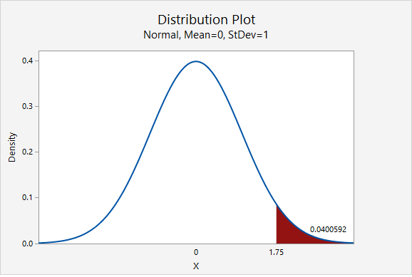
This is a right-tailed test so we need to find the area to the right of the test statistic, \(z=1.75\), on the z distribution.
Using Minitab , we find the probability \(P(z\geq1.75)=0.0400592\) which may be rounded to \(p\; value=0.0401\).
\(p\leq .05\), therefore our decision is to reject the null hypothesis
Yes, there is statistical evidence to state that more than 80% of all Americans are right handed.
8.1.2.1.3 - Example: Ice Cream
8.1.2.1.3 - Example: Ice CreamResearch Question: Is the percentage of Creamery customers who prefer chocolate ice cream over vanilla less than 80%?
In a sample of 50 customers 60% preferred chocolate over vanilla.
\(np_0 = 50(0.80) = 40\)
\(n(1-p_0)=50(1-0.80) = 10\)
Both \(np_0\) and \(n(1-p_0)\) are at least 10. We can use the normal approximation method.
This is a left-tailed test because we want to know if the proportion is less than 0.80.
\(H_{0}\colon p=0.80\)
\(H_{a}\colon p<0.80\)
- Test statistic: One Group Proportion
-
\(z=\dfrac{\widehat{p}- p_0 }{\sqrt{\frac{p_0 (1- p_0)}{n}}}\)
\(\widehat{p}\) = sample proportion
\(p_{0}\) = hypothesize population proportion
\(n\) = sample size
\(\widehat{p}=0.60\), \(p_{0}=0.80\), \(n=50\)
\(z= \dfrac{\widehat{p}- p_0 }{\sqrt{\frac{p_0 (1- p_0)}{n}}}= \dfrac{0.60-0.80}{\sqrt{\frac{0.80 (1-0.80)}{50}}}=-3.536\)
Our \(z\) test statistic is -3.536.
This is a left-tailed test so we need to find the area to the right of our test statistic, \(z=-3.536\).
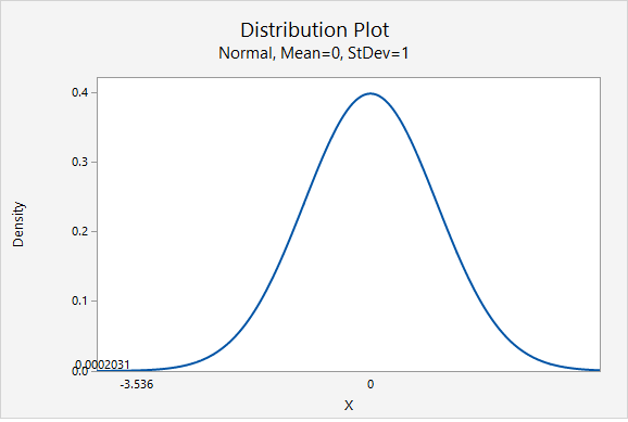
From the Minitab output above, the p-value is 0.0002031
\(p \leq.05\), therefore our decision is to reject the null hypothesis.
Yes, there is evidence that the percentage of all Creamery customers who prefer chocolate ice cream over vanilla is less than 80%.
8.1.2.1.4 - Example: Overweight Citizens
8.1.2.1.4 - Example: Overweight CitizensAccording to the Center for Disease Control (CDC), the percent of adults 20 years of age and over in the United States who are overweight is 69.0% (see http://www.cdc.gov/nchs/fastats/obesity-overweight.htm). One city’s council wants to know if the proportion of overweight citizens in their city is different from this known national proportion. They take a random sample of 150 adults 20 years of age or older in their city and find that 98 are classified as overweight. Let’s use the five step hypothesis testing procedure to determine if there is evidence that the proportion in this city is different from the known national proportion.
\(np_0 =150 (0.690)=103.5 \)
\(n (1-p_0) =150 (1-0.690)=46.5\)
Both \(n p_0\) and \(n (1-p_0)\) are at least 10, this assumption has been met.
Research question: Is this city’s proportion of overweight individuals different from 0.690?
This is a non-directional test because our question states that we are looking for a differences as opposed to a specific direction. This will be a two-tailed test.
\(H_{0}\colon p=0.690\)
\(H_{a}\colon p\neq 0.690\)
- Test statistic: One Group Proportion
-
\(z=\dfrac{\widehat{p}- p_0 }{\sqrt{\frac{p_0 (1- p_0)}{n}}}\)
\(\widehat{p}\) = sample proportion
\(p_{0}\) = hypothesize population proportion
\(n\) = sample size
\(\widehat{p}=\dfrac{98}{150}=.653\)
\( z =\dfrac{0.653- 0.690 }{\sqrt{\frac{0.690 (1- 0.690)}{150}}} = -0.980 \)
Our test statistic is \(z=-0.980\)
This is a non-directional (i.e., two-tailed) test, so we need to find the area under the z distribution that is more extreme than \(z=-0.980\).
In Minitab, we find the proportion of a normal curve beyond \(\pm0.980\):
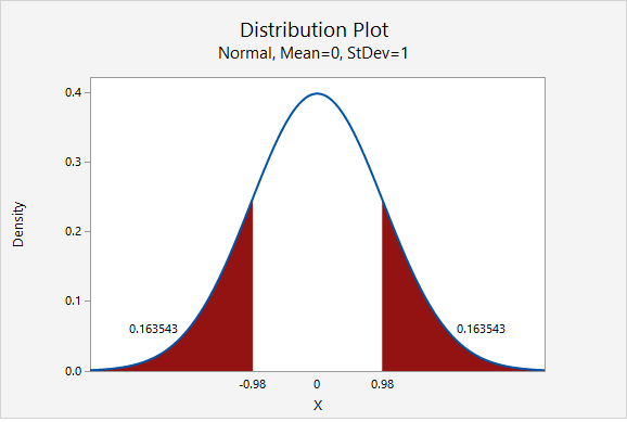
\(p-value=0.163543+0.163543=0.327086\)
\(p>\alpha\), therefore we fail to reject the null hypothesis
There is not sufficient evidence to state that the proportion of citizens of this city who are overweight is different from the national proportion of 0.690.
8.1.2.2 - Minitab: Hypothesis Tests for One Proportion
8.1.2.2 - Minitab: Hypothesis Tests for One ProportionA hypothesis test for one proportion can be conducted in Minitab. This can be done using raw data or summarized data.
- If you have a data file with every individual's observation, then you have raw data.
- If you do not have each individual observation, but rather have the sample size and number of successes in the sample, then you have summarized data.
The next two pages will show you how to use Minitab to conduct this analysis using either raw data or summarized data.
Note that the default method for constructing the sampling distribution in Minitab is to use the exact method. If \(np_0 \geq 10\) and \(n(1-p_0) \geq 10\) then you will need to change this to the normal approximation method. This must be done manually. Minitab will use the method that you select, it will not check assumptions for you!
8.1.2.2.1 - Minitab: 1 Proportion z Test, Raw Data
8.1.2.2.1 - Minitab: 1 Proportion z Test, Raw DataIf you have data in a Minitab worksheet, then you have what we call "raw data." This is in contrast to "summarized data" which you'll see on the next page.
In order to use the normal approximation method both \(np_0 \geq 10\) and \(n(1-p_0) \geq 10\). Before we can conduct our hypothesis test we must check this assumption to determine if the normal approximation method or exact method should be used. This must be checked manually. Minitab will not check assumptions for you.
In the example below, we want to know if there is evidence that the proportion of students who are male is different from 0.50.
\(n=226\) and \(p_0=0.50\)
\(np_0 = 226(0.50)=113\) and \(n(1-p_0) = 226(1-0.50)=113\)
Both \(np_0 \geq 10\) and \(n(1-p_0) \geq 10\) so we can use the normal approximation method.
Minitab® – Conducting a One Sample Proportion z Test: Raw Data
Research question: Is the proportion of students who are male different from 0.50?
- Open Minitab file:
- In Minitab, select Stat > Basic Statistics > 1 Proportion
- Select One or more samples, each in a column from the dropdown
- Double-click the variable Biological Sex to insert it into the box
- Check the box next to Perform hypothesis test and enter 0.50 in the Hypothesized proportion box
- Select Options
- Use the default Alternative hypothesis setting of Proportion ≠ hypothesized proportion value
- Use the default Confidence level of 95
- Select Normal approximation method
- Click OK and OK
The result should be the following output:
Method
Event: Biological Sex = Male
p: proportion where Biological Sex = Male
Normal approximation is used for this analysis.
| N | Event | Sample p | 95% CI for p |
|---|---|---|---|
| 226 | 99 | 0.438053 | (0.373368, 0.502738) |
| Null hypothesis | H 0: p = 0.5 |
|---|---|
| Alternative hypothesis | H 1: p ≠ 0.5 |
| Z-Value | P-Value |
|---|---|
| -1.86 | 0.063 |
Summary of Results
We could summarize these results using the five-step hypothesis testing procedure:
\(np_0 = 226(0.50)=113\) and \(n(1-p_0) = 226(1-0.50)=113\) therefore the normal approximation method will be used.
\(H_0\colon p = 0.50\)
\(H_a\colon p \ne 0.50\)
From the Minitab output, \(z\) = -1.86
From the Minitab output, \(p\) = 0.0625
\(p > \alpha\), fail to reject the null hypothesis
There is NOT enough evidence that the proportion of all students in the population who are male is different from 0.50.
8.1.2.2.2 - Minitab: 1 Sample Proportion z test, Summary Data
8.1.2.2.2 - Minitab: 1 Sample Proportion z test, Summary DataExample: Overweight
The following example uses a scenario in which we want to know if the proportion of college women who think they are overweight is less than 40%. We collect data from a random sample of 129 college women and 37 said that they think they are overweight.
First, we should check assumptions to determine if the normal approximation method or exact method should be used:
\(np_0=129(0.40)=51.6\) and \(n(1-p_0)=129(1-0.40)=77.4\) both values are at least 10 so we can use the normal approximation method.
Minitab® – Performing a One Proportion z Test with Summarized Data
To perform a one sample proportion z test with summarized data in Minitab:
- In Minitab, select Stat > Basic Statistics > 1 Proportion
- Select Summarized data from the dropdown
- For number of events, add 37 and for number of trials add 129.
- Check the box next to Perform hypothesis test and enter 0.40 in the Hypothesized proportion box
- Select Options
- Use the default Alternative hypothesis setting of Proportion < hypothesized proportion value
- Use the default Confidence level of 95
- Select Normal approximation method
- Click OK and OK
The result should be the following output:
Method
Event: Event proportion
Normal approximation is used for this analysis.
| N | Event | Sample p | 95% Upper Bound for p |
|---|---|---|---|
| 129 | 37 | 0.286822 | 0.352321 |
| Null hypothesis | H 0: p = 0.4 |
|---|---|
| Alternative hypothesis | H 1: p < 0.4 |
| Z-Value | P-Value |
|---|---|
| -2.62 | 0.004 |
Summary of Results
We could summarize these results using the five-step hypothesis testing procedure:
\(np_0=129(0.40)=51.6\) and \(n(1-p_0)=129(1-0.40)=77.4\) both values are at least 10 so we can use the normal approximation method.
\(H_0\colon p = 0.40\)
\(H_a\colon p < 0.40\)
From output, \(z\) = -2.62
From output, \(p\) = 0.004
\(p \leq \alpha\), reject the null hypothesis
There is evidence that the proportion of women in the population who think they are overweight is less than 40%.
8.1.2.2.2.1 - Minitab Example: Normal Approx. Method
8.1.2.2.2.1 - Minitab Example: Normal Approx. MethodExample: Gym membership
Research question: Are less than 50% of all individuals with a membership at one gym female?
A simple random sample of 60 individuals with a membership at one gym was collected. Each individual's biological sex was recorded. There were 24 females.
First we have to check the assumptions:
np = 60 (0.50) = 30
n(1-p) = 60(1-0.50) = 30
The assumptions are met to use the normal approximation method.
To perform a one sample proportion z test with summarized data in Minitab:
- In Minitab, select Stat > Basic Statistics > 1 Proportion
- Select Summarized data from the dropdown
- For number of events, add 24 and for number of trials add 60.
- Check the box next to Perform hypothesis test and enter 0.50 in the Hypothesized proportion box
- Select Options
- Use the default Alternative hypothesis setting of Proportion < hypothesized proportion value
- Use the default Confidence level of 95
- Select Normal approximation method
- Click OK and OK
The result should be the following output:
Method
Event: Event proportion
Normal approximation is used for this analysis.
| N | Event | Sample p | 95% Upper Bound for p |
|---|---|---|---|
| 60 | 24 | 0.400000 | 0.504030 |
| Null hypothesis | H 0: p = 0.5 |
|---|---|
| Alternative hypothesis | H 1: p < 0.5 |
| Z-Value | P-Value |
|---|---|
| -1.55 | 0.061 |
We could summarize these results using the five-step hypothesis testing procedure:
\(np_0=60(0.50)=30\) and \(n(1-p_0)=60(1-0.50)=30\) both values are at least 10 so we can use the normal approximation method.
\(H_0\colon p = 0.50\)
\(H_a\colon p < 0.50\)
From output, \(z\) = -1.55
From output, \(p\) = 0.061
\(p \geq \alpha\), fail to reject the null hypothesis
There is not enough evidence to support the alternative that the proportion of women memberships at this gym is less than 50%.
8.2 - One Sample Mean
8.2 - One Sample MeanOne sample mean tests are covered in Section 6.2 of the Lock5 textbook.
Concerning one sample mean, the Central Limit Theorem states that if the sample size is large, then the distribution of sample means will be approximately normally distributed with a standard deviation (i.e., standard error) equal to \(\frac{\sigma}{\sqrt n}\). In this course, a "large" sample size will be defined as one where \(n \ge 30\).
When constructing confidence interval and conducting hypothesis tests we often do not know the value of \(\sigma\). In those cases, \(\sigma\) may be estimated using the sample standard deviation (\(s\)). When we are using \(s\) to estimate \(\sigma\) our sampling distribution will not follow a \(z\) distribution exactly. Instead, we use what is known as the \(t\) distribution. Like the \(z\) distribution, the \(t\) distribution is symmetrical. The difference is that its height varies depending on the sample size. By doing so, the distribution becomes more conservative for smaller sample sizes to account for some error that may occur from estimating \(\sigma\) with \(s\) from a small sample. As \(n\) approaches infinity (\(\infty\)) the \(t\) distribution approaches the standard normal distribution. The next page compares the \(z\) and \(t\) distributions.
When constructing confidence intervals and conducting hypothesis tests we will usually be using the \(t\) distribution when working with one mean. The only exception would be in cases where \(\sigma\) is known. This scenario is most common in the fields of education and psychology where some tests are normed to have a certain \(\mu\) and \(\sigma\). In those cases, the \(z\) distribution can be used.
In terms of language, all of these tests could be called "single sample mean tests" or "one sample mean tests." We could also specify the sampling distribution by using the term "single sample mean \(t\) test" or "single sample mean \(z\) test."
The flow chart below may help you in determining which method should be used when constructing a sampling distribution for one sample mean.
One Sample Mean
Identify when z and t distributions should be used.
- Is the population known to be normally distributed?
- Is the population standard deviation known?
- Is the sample size at least 30?
8.2.1 - t Distribution
8.2.1 - t DistributionThe height of the t distribution is determined by the number of degrees of freedom (df). For a one sample mean test, \(df=n-1\).
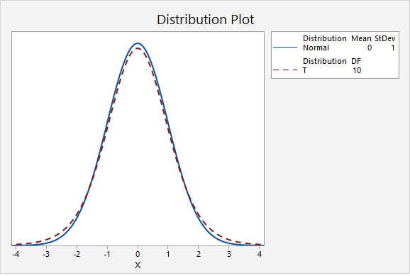
The first plot below compares the standard normal distribution (i.e., z distribution) to a t distribution. The solid blue line is the standard normal distribution and the dashed red line is a t distribution with 2 degrees of freedom. Here, the tails of the t distribution are higher than the tails of the normal distribution.
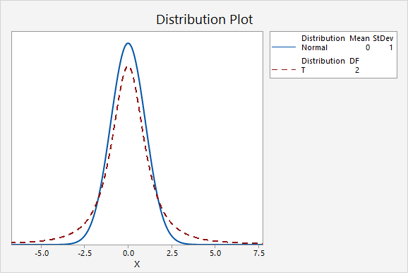
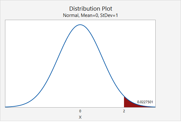
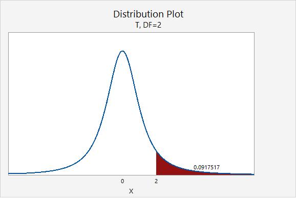
If you think about the area under the curve, the higher tails mean that more area will fall in the tails. For example, as seen in the following two plots, \(P(z>2.00)=0.0227501\) while \(P(t_{df=2}>2.00)=0.0917517\).
The next plot compares the standard normal distribution to a t distribution with 10 degrees of freedom. Notice that the two distributions are becoming more similar as the sample size increases.
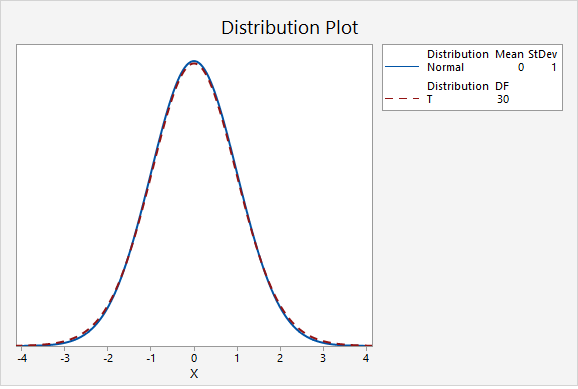
The next plot compares the standard normal distribution to a t distribution with 30 degrees of freedom.
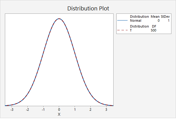
In the final graph, the standard normal distribution is compared to a t distribution with 500 degrees of freedom. Here, the two distributions are nearly identical. As the degrees of freedom approach infinity, the t distribution approaches (i.e., becomes more similar to) the standard normal distribution.
Minitab®
The procedures for constructing t distributions in Minitab are similar to those for constructing z distributions. We can construct a probability distribution plot to find the t* multiplier when constructing a confidence interval. And, we can construct a plot to find the p-value when conducting a hypothesis test.
Steps for finding the t* multiplier
- In Minitab, select Graph > Probability Distribution Plot > View Probability
- Change the Distribution to t
- Enter your Degrees of freedom
- Select Options
- Choose A specified probability
- Select Equal tails
- For Probability enter the value that is split between the two tails (e.g., for a 90% confidence interval you would enter 0.10)
Steps for finding the p value given a t test statistic
- In Minitab, select Graph > Probability Distribution Plot > View Probability
- Change the Distribution to t
- Enter your Degrees of freedom
- Select A specified x value
- Select Right tail, Left tail, or Equal tails, depending on the direction of your alternative hypothesis
- For X value enter the t test statistic
8.2.2 - Confidence Intervals
8.2.2 - Confidence IntervalsConfidence intervals are used to estimate unknown population parameters. Because the population standard deviation (\(\sigma\)) will almost always be unknown in situations in which we are constructing confidence intervals for means, the \(t\) distribution is used to estimate the sampling distribution. The following pages will show you how to construct a confidence interval for a population mean using formulas and using Minitab. Similar to how we computed necessary minimum sample sizes for confidence intervals for proportions, we will also compute the necessary minimum sample size for constructing a confidence interval for a mean.
8.2.2.1 - Formulas
8.2.2.1 - FormulasEarlier in this lesson we considered confidence intervals for proportions and the multiplier in our intervals was a value from the standard normal (i.e., \(z\)) distribution. But, what if our variable of interest is a quantitative variable and we want to estimate a population mean?
We apply similar techniques when constructing a confidence interval for a mean, but now we are interested in estimating the population mean (\(\mu\)) by using the sample statistic (\(\overline{x}\)) and the multiplier is a \(t\) value. Similar to the \(z\) values that you used as the multiplier for constructing confidence intervals for population proportions, here you will use \(t\) values as the multipliers. Because \(t\) values vary depending on the number of degrees of freedom (df), you will need to use statistical software to look up the appropriate \(t\) value for each confidence interval that you construct. The degrees of freedom will be based on the sample size. Since we are working with one sample here, \(df=n-1\).
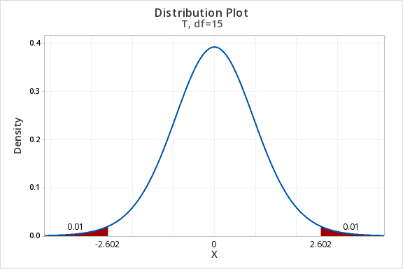
Minitab® – Finding t* Multipliers
To find the t* multiplier for a 98% confidence interval with 15 degrees of freedom:
- In Minitab, select Graph > Probability Distribution Plot > View Probability
- Change the Distribution to t
- Enter 15 for the Degrees of freedom
- Select Options
- Choose A specified probability
- Select Equal tails
- For Probability enter 0.02 (if there is 0.98 in the middle, then 0.02 is split equally between the left and right tails)
This should result in an output similar to the output below. Note that your results may be slightly different due to random sampling variation.
Let’s review some of symbols and equations that we learned in previous lessons:
| Sample size | \(n\) |
|---|---|
| Population mean | \(\mu=\frac{\sum X}{N}\) |
| Sample mean | \(\overline{x}= \frac{\sum x}{n}\) |
| Standard error of the mean | \(SE=\frac{s}{\sqrt{n}}\) |
| Multiplier | \(t^{*} \) |
| Degrees of freedom (one group) | \(df=n-1\) |
Recall the general form for a confidence interval:
- General Form of Confidence Interval
- \(sample\ statistic\pm\underbrace{(multiplier)\ (standard\ error)}_{\textbf{margin of error}}\)
When constructing a confidence interval for a population mean the point estimate is the sample mean, \(\overline{x}\). The multiplier is taken from a \(t\) distribution. And, the standard error is equal to \(\frac{s}{\sqrt{n}}\).
- Confidence Interval for a Population Mean
- \(\underbrace{\overline{x}}_{\text{sample statistic}} \pm \overbrace{t^{*}}^{\text{multiplier}} \underbrace{ \dfrac{s}{\sqrt{n}}}_{\text{standard error}}\)
On the following pages we will walk through examples of constructing confidence intervals for population means by hand. Then, you will learn how to compute confidence intervals using Minitab.
8.2.2.1.1 - Example: MLB Age
8.2.2.1.1 - Example: MLB AgeIn a sample of 30 current MLB pitchers, the mean age was 28 years with a standard deviation of 4.4 years. Construct a 95% confidence interval to estimate the mean age of all current MLB pitchers.
This is what we know: \(n=30\), \(\overline{x}=28\), and \(s=4.4\).
In order to compute the confidence interval for \(\mu\) we will need the t multiplier and the standard error (\( \frac{s}{\sqrt{n}}\)).
\(df=n-1=30-1=29\)
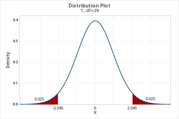
For a 95% confidence interval with 29 degrees of freedom, \(t^{*}=2.045\)
\(SE=\dfrac{s}{\sqrt{n}}=\dfrac{4.4}{\sqrt{30}}=0.803\)
Thus, our confidence interval for \(\mu\) is: \(28\pm 2.045(0.803)=28\pm1.643=[26.357,29.643]\)
We are 95% confident that the population mean age is between 26.357 and 29.643.
8.2.2.1.2- Example: Sleep Deprivation
8.2.2.1.2- Example: Sleep DeprivationIn a class survey, students were asked how many hours they sleep per night. In the sample of 22 students, the mean was 5.77 hours with a standard deviation of 1.572 hours. That distribution was approximately normal. Let’s construct a 95% confidence interval for the mean number of hours slept per night in the population from which this sample was drawn.
This is what we know: \(n=22\), \(\overline{x}=5.77\), and \(s=1.572\).
In order to compute the confidence interval for \(\mu\) we will need the t multiplier and the standard error (\( \frac{s}{\sqrt{n}}\)).
\(df=n-1=22-1=21\)
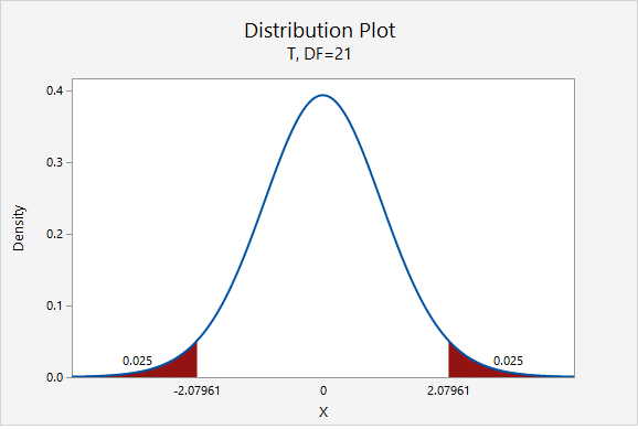
For a 95% confidence interval with 21 degrees of freedom, \(t^{*}=2.080\)
\(SE=\frac{s}{\sqrt{n}}=\frac{1.572}{\sqrt{22}}=0.335\)
Thus, our confidence interval for \(\mu\) is: \(5.77\pm 2.080(0.335)=5.77\pm0.697=[5.073,\;6.467]\)
We are 95% confident that the population mean is between 5.073 and 6.467 hours.
The only thing that would change is our multiplier. Now, \(t^{*}=2.831\).
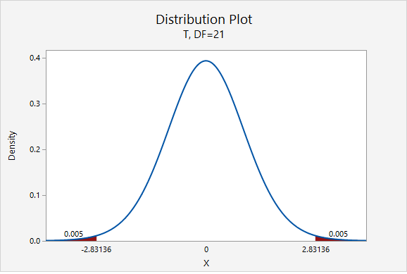
\(5.77\pm 2.831(0.335)=5.77\pm0.948=[4.822,\;6.718]\)
We are 99% confident that the population mean is between 4.822 and 6.718 hours.
8.2.2.1.3 - Example: Milk
8.2.2.1.3 - Example: MilkA study of 66,831 dairy cows found that the mean milk yield was 12.5 kg per milking with a standard deviation of 4.3 kg per milking (data from Berry, et al., 2013). Construct a 95% confidence interval for the average milk yield in the population.
First, let's compute the standard error:
\(SE=\dfrac{s}{\sqrt{n}}=\dfrac{4.3}{\sqrt{66831}}=0.0166\)
The standard error is small because the sample size is very large.
Next, let's find the \(t^*\) multiplier:
\(df=66831-1=66830\)
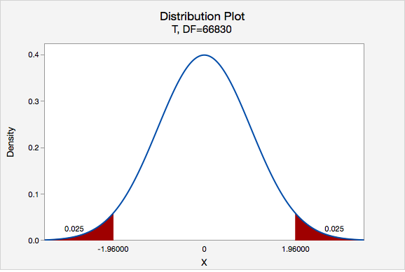
\(t^{*}=1.960\)
Now, we can construct our 95% confidence interval:
95% C.I.: \(12.5\pm1.960(0.017)=12.5\pm0.033=[12.467,\;12.533]\)
We are 95% confident that the mean milk yield in the population is between 12.467 and 12.533 kg per milking.
8.2.2.2 - Minitab: Confidence Interval of a Mean
8.2.2.2 - Minitab: Confidence Interval of a MeanHere you will learn how to use Minitab to construct a confidence interval for a mean. The procedure is similar to the one that you learned earlier in this lesson for constructing a confidence interval for a proportion. The following example walks through this procedure when data are in a Minitab work. At the bottom of this page you will find instructions for using Minitab with summarized data.
Minitab® – Confidence Interval for a Mean
To create a 95% confidence interval of mean height in Minitab:
- Open the data set: fall2016stdata.csv
- In Minitab, select Stat > Basic Statistics > 1-sample t
- In this case we have our data in the Minitab worksheet so we will use the default One or more samples, each in a column
- Double click the variable Height in the box on the left to insert the variable into the box
- Select Options
- The default Confidence level is 95
- Click OK and OK
This should result in the following output:
| N | Mean | StDev | SE Mean | 95% CI for \(\mu\) |
|---|---|---|---|---|
| 525 | 67.009 | 4.462 | 0.195 | (66.627, 67.392) |
\(\mu\): mean of Height
What if we have summarized data and not data in a Minitab worksheet?
If you do not have a Minitab worksheet filled with data concerning individuals, but instead have summarized data (e.g., the values of \(s\), \(\overline{x}\), and \(n\)), you would skip step 1 above and in step 3 you would select Summarized data.
8.2.2.2.1 - Example: Age of Pitchers (Summarized Data)
8.2.2.2.1 - Example: Age of Pitchers (Summarized Data)Example: Estimating the average MLB Pitcher's age
In a sample of 30 current MLB pitchers, the mean age was 28 years with a standard deviation of 4.4 years. Construct a 95% confidence interval to estimate the mean age of all current MLB pitchers.
We know that n = 30, \(\bar{x}=28\), and s = 4.4.
To create a 95% confidence interval of mean age in Minitab:
- In Minitab, select Stat > Basic Statistics > 1-sample t
- In this case we have summarized data so select Summarized Data from the dropdown
- Enter 30 for the sample size, 28 for the sample mean and 4.4 for the standard deviation.
- Select Options
- The default Confidence level is 95
- Click OK and OK
This should result in the following output:
| N | Mean | StDev | SE Mean | 95% CI for \(\mu\) |
|---|---|---|---|---|
| 30 | 28.000 | 4.400 | 0.803 | (26.357, 29.643) |
\(\mu\): population mean of sample
We are 95% confident that the population mean age is between 26.357 and 29.643 years.
8.2.2.2.2 - Example: Coffee Sales (Data in Column)
8.2.2.2.2 - Example: Coffee Sales (Data in Column)For 48 days data concerning sales were collected from one student-run cafe. Let's construct a 95% confidence interval for the mean number of coffees sold per day.
To create a 95% confidence interval of mean number of coffees sold per day in Minitab:
- Open the file: cafedata.mpx
- In Minitab, select Stat > Basic Statistics > 1-sample t
- In this case the data is in a worksheet so select use One or more samples, each in a column
- Select the variable Coffees
- Select Options
- The default Confidence level is 95
- Click OK and OK
This should result in the following output:
| N | Mean | StDev | SE Mean | 95% CI for \(\mu\) |
|---|---|---|---|---|
| 47 | 21.51 | 11.08 | 1.62 | (18.26, 24.76) |
\(\mu\): population mean of Coffees
We are 95% confident that the population mean number of coffees solder per day is between 18.26 and 24.76.
8.2.2.3 - Computing Necessary Sample Size
8.2.2.3 - Computing Necessary Sample SizeCalculating the sample size necessary for estimating a population mean with a given margin of error and level of confidence is similar to that for estimating a population proportion. However, since the \(t\) distribution is not as “neat” as the standard normal distribution, the process can be iterative. (Recall, the shape of the \(t\) distribution is different for each degree of freedom). This means that we would solve, reset, solve, reset, etc. until we reached a conclusion. Yet, we can avoid this iterative process if we employ an approximate method based on \(t\) distribution approaching the standard normal distribution as the sample size increases. This approximate method invokes the following formula:
- Finding the Sample Size for Estimating a Population Mean
- \(n=\dfrac{z^{2}\widetilde{\sigma}^{2}}{M^{2}}=\left ( \dfrac{z\widetilde{\sigma}}{M} \right )^2\)
-
\(z\) = z multiplier for given confidence level
\(\widetilde{\sigma}\) = estimated population standard deviation
\(M\) = margin of error
The sample standard deviation may be estimated on the basis of prior research studies.
8.2.2.3.1 - Example: Estimating IQ
8.2.2.3.1 - Example: Estimating IQExample: Estimating IQ
A team of researchers wants to estimate the mean IQ of students enrolled at one prestigious university. Previous research studies have examined samples of students from other similar universities and usually find results around \(\overline{x}=120\) and \(s=10\). In order to construct a 90% confidence interval with a margin of error of \(\pm2\) IQ points, what sample size should be obtained?
As shown in the probability distribution plot below, the z value associated with a 90% confidence interval is 1.645.
The estimated standard deviation is given to be 10 and the desired margin of error is given to be 2.
\(n=\dfrac{z^{2}\widetilde{\sigma}^{2}}{M^{2}}=\dfrac{1.645^{2}(10^{2})}{2^{2}}=67.615\)
We round up to 68. The research team should attempt to obtain a sample of at least 68 individuals.
8.2.2.3.2 - Video Example: Age
8.2.2.3.2 - Video Example: Age8.2.2.3.3 - Video Example: Cookie Weights
8.2.2.3.3 - Video Example: Cookie Weights8.2.3 - Hypothesis Testing
8.2.3 - Hypothesis TestingIn this section we will be comparing one sample mean to one known or hypothesized population value. In Lesson 5 you learned how to conduct randomization tests. Here, you will learn how to conduct a one sample mean \(t\) test and a one sample mean \(z\) test. The \(t\) distribution is used to estimate the sampling distribution when the sample size is large (at least 30) or when the population is known to be normally distributed (but \(\sigma\) is unknown). The \(z\) distribution is used on rare occasions when the population is normal and the population standard deviation is known. Note that for this course the one sample mean \(z\) test is optional; it used only in specific cases where the population is known to be normally distributed and when the population standard deviation (\(\sigma\)) is known. The most commonly used one sample mean test is the "one sample mean \(t\) test" which is also known as a "single sample mean \(t\) test."
8.2.3.1 - One Sample Mean t Test, Formulas
8.2.3.1 - One Sample Mean t Test, Formulas
Five Step Hypothesis Testing Procedure
Data must be quantitative. In order to use the t distribution to approximate the sampling distribution either the sample size must be large (\(\ge\ 30\)) or the population must be known to be normally distributed. The possible combinations of null and alternative hypotheses are:
| Research Question | Is the mean different from \( \mu_{0} \)? | Is the mean greater than \(\mu_{0}\)? | Is the mean less than \(\mu_{0}\)? |
|---|---|---|---|
| Null Hypothesis, \(H_{0}\) | \(\mu=\mu_{0} \) | \(\mu=\mu_{0} \) | \(\mu=\mu_{0} \) |
| Alternative Hypothesis, \(H_{a}\) | \(\mu\neq \mu_{0} \) | \(\mu> \mu_{0} \) | \(\mu<\mu_{0} \) |
| Type of Hypothesis Test | Two-tailed, non-directional | Right-tailed, directional | Left-tailed, directional |
where \( \mu_{0} \) is the hypothesized population mean.
For the test of one group mean we will be using a \(t\) test statistic:
- Test Statistic: One Group Mean
-
\(t=\dfrac{\overline{x}-\mu_0}{\frac{s}{\sqrt{n}}}\)
\(\overline{x}\) = sample mean
\(\mu_{0}\) = hypothesized population mean
\(s\) = sample standard deviation
\(n\) = sample size
Note that structure of this formula is similar to the general formula for a test statistic:
\(\dfrac{sample\;statistic-null\;value}{standard\;error}\)
When testing hypotheses about a mean or mean difference, a \(t\) distribution is used to find the \(p\)-value. These \(t\) distributions are indexed by a quantity called degrees of freedom, calculated as \(df = n – 1\) for the situation involving a test of one mean or test of mean difference. The \(p\)-value can be found using Minitab.
If \(p \leq \alpha\) reject the null hypothesis.
If \(p>\alpha\) fail to reject the null hypothesis.
Based on your decision in Step 4, write a conclusion in terms of the original research question.
The new few pages will walk you through examples before giving you the opportunity to do two on your own.
8.2.3.1.1 - Video Example: Book Costs
8.2.3.1.1 - Video Example: Book CostsResearch question: Does the average Penn State student spend more than \$300 each semester on textbooks?
In a sample of 226 Penn State students, the mean cost of a student’s textbooks was \$344 with a standard deviation of \$106.
8.2.3.1.2 : Example: Pulse Rate
8.2.3.1.2 : Example: Pulse RateA research study measured the pulse rates of 57 college men and found a mean pulse rate of 70.4211 beats per minute with a standard deviation of 9.9480 beats per minute. Researchers want to know if the mean pulse rate for all college men is different from the current standard of 72 beats per minute.
Pulse rates are quantitative. The sampling distribution will be approximately normally distributed because \(n \ge 30\).
This is a two-tailed test because we want to know if the mean pulse rate is different from 72.
\(H_{0}:\mu=72 \)
\(H_{a}: \mu\neq 72 \)
- Test Statistic: One Group Mean
-
\(t=\dfrac{\overline{x}-\mu_0}{\dfrac{s}{\sqrt{n}}}\)
\(\overline{x}\) = sample mean
\(\mu_{0}\) = hypothesized population mean
\(s\) = sample standard deviation
\(n\) = sample size
\(t=\dfrac{\overline{x}-\mu_0}{\dfrac{s}{\sqrt{n}}}=\dfrac{70.4211-72}{\dfrac{9.9480}{\sqrt{57}}}=-1.198\)
Our \(t\) test statistic is -1.198
\(df=n-1=57-1=56\)
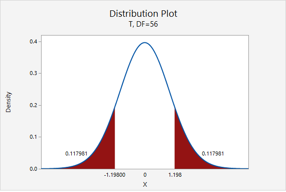
\(p=0.117981+0.117981=0.235962\)
Given that the null hypothesis is true and \(\mu=72\), the probability of taking a random sample of \(n=57\) and finding a sample mean this or more extremely different is 0.235962. This is our p-value.
\(p>.05\), therefore we fail to reject the null hypothesis.
There is not sufficient evidence to state that the mean pulse of college men is different from 72.
8.2.3.1.3 - Example: Coffee
8.2.3.1.3 - Example: CoffeeIn the population of Americans who drink coffee, the average daily consumption is 3 cups per day. A university wants to know if their students tend to drink more coffee than the national average. They ask a random sample of 50 students how many cups of coffee they drink each day and found \(\overline{x}=3.8\) and \(s=1.5\). Do they have evidence that their students drink more than the national average?
Amount of coffee consumed is a quantitative variable. We are given that random sampling methods were employed. Because \(n \ge 30\), we can approximate the sampling distribution using a t distribution.
This is a right-tailed test because we want to know if the mean in the sample is greater than the national average.
\(H_{0}:\mu= 3\)
\(H_{a}:\mu>3\)
- Test Statistic: One Group Mean
-
\(t=\dfrac{\overline{x}-\mu_0}{\dfrac{s}{\sqrt{n}}}\)
\(\overline{x}\) = sample mean
\(\mu_{0}\) = hypothesized population mean
\(s\) = sample standard deviation
\(n\) = sample size
\(t=\dfrac{\overline{x}-\mu_0}{\dfrac{s}{\sqrt{n}}}=\dfrac{3.8-3}{\dfrac{1.5}{\sqrt{50}}}=3.771\)
Our \(t\) test statistic is 3.771
\(df=n-1=50-1=49\)
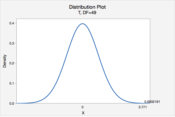
Using Minitab, we can find that \(P(t > 3.771) =0.0002191\)
p-value = 0.0002191
If \(\mu=3\), then the probability of taking a random sample of \(n=50\) and finding \(\overline{x} \geq 3\) is 0.0002191
\(p\leq.05\), therefore we reject the null hypothesis.
There is evidence to state the mean number of coffees consumed in the population of all students at this university is greater than 3.
8.2.3.1.4 - Example: Transportation Costs
8.2.3.1.4 - Example: Transportation CostsAccording to CNN, in 2011, the average American spent \$16,803 on housing. A suburban community wants to know if their residents spent less than this national average. In a survey of 30 randomly selected residents, they found that they spent an annual average of \$15,800 with a standard deviation of \$2,600.
Housing costs are quantitative. Because \(n \ge 30\), the sampling distribution can be approximated using the \(t\) distribution.
This is a left-tailed test because we want to know if residents of this community spent less than the national average.
\(H_{0}:\mu=16803\)
\(H_{a}:\mu<16803\)
- Test Statistic: One Group Mean
-
\(t=\dfrac{\overline{x}-\mu_0}{\dfrac{s}{\sqrt{n}}}\)
\(\overline{x}\) = sample mean
\(\mu_{0}\) = hypothesized population mean
\(s\) = sample standard deviation
\(n\) = sample size
\(t=\dfrac{\overline{x}-\mu_0}{\dfrac{s}{\sqrt{n}}}=\dfrac{15800-16803}{\dfrac{2600}{\sqrt{30}}}=-2.113\)
Our t test statistics is -2.113
\(df=n-1=30-1=29\)
This is a left-tailed test so we want to know the probability of \(t < -2.113\)
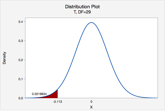
Using Minitab we can find that \(p=0.0216634\)
\(p\leq .05\), therefore we reject the null hypothesis.
There is evidence to state that on average residents of this community spent less than the national average on housing in 2011.
8.2.3.2 - Minitab: One Sample Mean t Tests
8.2.3.2 - Minitab: One Sample Mean t TestsA hypothesis test for one group mean can be conducted in Minitab using raw data or summarized data.
- If you have a data file with every individual's observation, then you have raw data.
- If you do not have each individual's observation, but rather have the sample mean, sample standard deviation, and sample size, then you have summarized data.
The next two pages will show you how to use Minitab to conduct a one-sample mean t-test using either raw data or summarized data. There is also one example of using Minitab to conduct a one-sample mean z test which is only performed if the population is known to be normally distributed and the population standard deviation (\(\sigma\)) is available.
8.2.3.2.1 - Minitab: 1 Sample Mean t Test, Raw Data
8.2.3.2.1 - Minitab: 1 Sample Mean t Test, Raw DataMinitab® – One Sample Mean t Test Using Raw Data
Research question: Is the mean GPA in the population different from 3.0?
- Null hypothesis: \(\mu\) = 3.0
- Alternative hypothesis: \(\mu\) ≠ 3.0
The GPAs of 226 students are available.
A one sample mean \(t\) test should be performed because the shape of the population is unknown, however the sample size is large (\(n\) ≥ 30).
To perform a one sample mean \(t\) test in Minitab using raw data:
- Open the Minitab file: class_survey.mpx
- Select Stat > Basic Statistics > 1-sample t
- Select One or more samples, each in a column from the dropdown
- Double-click on the variable GPA to insert it into the Sample box
- Check the box Perform a hypothesis test
- For the Hypothesized mean enter 3
- Select Options
- Use the default Alternative hypothesis of Mean ≠ hypothesized value
- Use the default Confidence level of 95
- Click OK and OK
This should result in the following output:
| N | Mean | StDev | SE Mean | 95% CI for \(\mu\) |
|---|---|---|---|---|
| 226 | 3.2311 | 0.5104 | 0.0340 | (3.1642, 3.2980) |
| Null hypothesis | H0: \(\mu\) = 3 |
|---|---|
| Alternative hypothesis | H1: \(\mu\) ≠ 3 |
| T-Value | P-Value |
|---|---|
| 6.81 | 0.000 |
Summary of Results
We could summarize these results using the five step hypothesis testing procedure:
We do not know if the population is normally distributed, however the sample size is large (\(n \ge 30\)) so we can perform a one sample mean t test.
\(H_0\colon \mu = 3.0\)
\(H_a\colon \mu \ne 3.0\)
\(t (225) = 6.81\)
\(p < 0.0001\)
\(p \le \alpha\), reject the null hypothesis
There is evidence that the mean GPA in the population is different from 3.0
8.2.3.2.2 - Minitab: 1 Sample Mean t Test, Summarized Data
8.2.3.2.2 - Minitab: 1 Sample Mean t Test, Summarized DataMinitab® – One Sample Mean t Test Using Summarized Data
Here we are testing \(H_{a}\colon\mu\neq72\) and are given \(n=35\), \(\bar{x}=76.8\), and \(s=11.62\).
We do not know the shape of the population, however the sample size is large (\(n \ge 30\)) therefore we can conduct a one sample mean \(t\) test.
To perform a one sample mean \(t\) test in Minitab using raw data:
- In Minitab, select Stat > Basic Statistics > 1-sample t
- Select Summarized data from the dropdown
- Enter 35 for the sample size, 76.8 for the sample mean and 11.62 for the standard deviation.
- Check the box Perform a hypothesis test
- For the Hypothesized mean enter 72
- Select Options
- Use the default Alternative hypothesis of Mean ≠ hypothesized value
- Use the default Confidence level of 95
- Click OK and OK
This should result in the following output:
Descriptive Statistics
| N | Mean | StDev | SE Mean | 95% CI for \(\mu\) |
|---|---|---|---|---|
| 35 | 76.80 | 11.62 | 1.96 | (72.81, 80.79) |
| Null hypothesis | H0: \(\mu\) = 72 |
|---|---|
| Alternative hypothesis | H1: \(\mu\) ≠ 72 |
| T-Value | P-Value |
|---|---|
| 2.44 | 0.0199 |
We could summarize these results using the five step hypothesis testing procedure:
The shape of the population distribution is unknown, however with \(n \ge 30\) we can perform a one sample mean t test.
\(H_0\colon \mu = 72\)
\(H_a\colon \mu \ne 72\)
\(t (34) = 2.44\)
\(p = 0.0199\)
\(p \le \alpha\), reject the null hypothesis
There is evidence that the population mean is different from 72.
8.2.3.3 - One Sample Mean z Test (Optional)
8.2.3.3 - One Sample Mean z Test (Optional)A one sample mean \(z\) test is used when the population is known to be normally distributed and when the population standard deviation (\(\sigma\)) is known. This most frequently occurs in the social sciences when standardized measures are used such as IQ, SAT, ACT, or GRE scores, for which the population parameters are known.
The formula for computing a \(z\) test statistic for one sample mean is identical to that of computing a \(t\) test statistic for one sample mean, except now the population standard deviation is known and can be used in computing the standard error.
- z Test Statistic: One Group Mean
- \(z=\dfrac{\overline{x}-\mu_0}{\dfrac{\sigma}{\sqrt{n}}}\)
-
\(\overline{x}\) = sample mean
\(\mu_{0}\) = hypothesized population mean
\(s\) = sample standard deviation
\(n\) = sample size
The other primary difference between the one sample mean \(t\) test and the one sample mean \(z\) test is the latter uses the standard normal distribution (i.e., \(z\) distribution) in determining the \(p\)-value. Below are the directions for conducting a one sample mean \(z\) test in Minitab.
Minitab® – Performing a One Sample Mean z Test
Research question: Are the IQ scores of students at one college-prep school above the national average?
Scores on one American IQ test are normed to have a mean of 100 and standard deviation of 15. In a simple random sample of 25 students at this school the mean was 110.
To perform a one-sample mean z test in Minitab using summarized data:
- In Minitab, select Stat > Basic Statistics > 1-sample Z
- Select Summarized data from the dropdown
- Enter 25 for the sample size, 110 for the sample mean and 15 for the known standard deviation.
- Check the box Perform a hypothesis test
- For the Hypothesized mean enter 100
- Select Options
- Use the default Alternative hypothesis of Mean > hypothesized value
- Use the default Confidence level of 95
- Click OK and OK
This should result in the following output:
Descriptive Statistics
| N | Mean | SE Mean | 95% Lower Bound for \(\mu\) |
|---|---|---|---|
| 25 | 110.00 | 3.00 | 105.07 |
\(\mu\): population mean of Sample
Known standard deviation = 15
Test
| Null hypothesis | H0: \(\mu\) = 100 |
|---|---|
| Alternative hypothesis | H1: \(\mu\) > 100 |
| Z-Value | P-Value |
|---|---|
| 3.33 | 0.000 |
Summary of Results
We could summarize these results using the five step hypothesis testing procedure:
The population is known to be normally distributed and the population standard deviation is known to be 15. With these two conditions met we can conduct a one sample mean z test
\(H_0\colon \mu = 100\)
\(H_a\colon \mu > 100\)
From the Minitab output, \(z = 3.33\)
From the Minitab output, \(p = 0.000\)
\(p \le \alpha\), reject the null hypothesis
There is evidence that the mean IQ score of all students at this school is greater than 100.
8.3 - Paired Means
8.3 - Paired MeansIn Lesson 1 we learned about independent samples and paired samples. When we have two independent samples, the observations in the two groups are unrelated to one another and are not matched in any meaningful way. We'll learn how to compare the means of two independent groups in Lesson 9.
With paired samples, the observations in the two groups are matched in a meaningful way. These are also known as dependent samples. Most often this occurs when data are collected twice from the same participants, called repeated measures. For example, think of studying the effectiveness of a diet plan. You would weigh each participant prior to starting the diet and again following some time on the diet. Depending on how much weight they lost you would determine if the diet was effective. Paired data does not always need to involve two measurements on the same subject; it can also involve taking one measurement on each of two related subjects. For example, we may study husband-wife pairs, mother-son pairs, or pairs of twins.
In constructing a dependent samples confidence interval or conducting a dependent samples hypothesis test, the difference score is computed for each individual or pair. From there, the procedures are the same that you used for constructing confidence intervals and hypothesis tests for single sample means. As with one sample mean, if the sample size is at least 30, the sampling distribution for the difference in paired means can be approximated using a \(t\) distribution.
In terms of symbols, the population parameter of interest is the mean difference in the population "\(\mu_d\)." This is estimated using the mean difference in the sample "\(\overline x_d\)."
8.3.1 - Confidence Intervals
8.3.1 - Confidence IntervalsRecall the general form of a confidence interval...
\(sample\ statistic\pm\underbrace{(multiplier)\ (standard\ error)}_{\textbf{margin of error}}\).
The formula for constructing a confidence interval for the difference in paired means is almost identical to the formula for constructing a confidence interval for one mean. Note that the only change is the subscript d which stands for difference.
Confidence Interval for the Difference Between Two Paired Means
\(\underbrace{\overline{x}_d}_{\text{sample statistic}} \pm \overbrace{t^*}^{\text{multiplier}} \underbrace{\left(\dfrac{s_d}{\sqrt{n}}\right)}_{\text{standard error}}\)
\(t^*\) is the multiplier with \(df = n-1\)
8.3.1.1. - Example: Change in Knowledge
8.3.1.1. - Example: Change in KnowledgeAn educational research study is designed so that participants complete a measure of demonstrated knowledge twice. The researcher wants to estimate the change in scores from the first to second administrations (i.e., pre- and post-test). Data are paired by participant. The researcher subtracted pre-test scores from the post test scores and found a mean increase of 6.560 with a standard deviation of 3.867 for \(n=100\). She wants to construct a 95% confidence interval for the mean difference.
First, we'll find the appropriate multiplier.
\(df=n-1=100-1=99\)
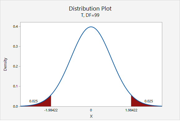
For a 95% confidence interval: \(t_{df=99}=1.984\)
\(6.560 \pm 1.984 \left(\frac{3.867}{\sqrt{100}}\right)=6.560 \pm 0.767=[5.793, 7.327]\)
We are 95% confident that the difference between post- and pre- test scores is between 5.793 and 7.327.
Data from Zimmerman, W. A. (2015). Impact of Instructional Materials Eliciting Low and High Cognitive Load on Self-Efficacy and Demonstrated Knowledge (Unpublished doctoral dissertation). The Pennsylvania State University, University Park, PA.
8.3.1.2 - Video Example: Difference in Exam Scores
8.3.1.2 - Video Example: Difference in Exam Scores8.3.2 - Hypothesis Testing
8.3.2 - Hypothesis TestingBelow are the procedures for conducting a hypothesis test for two paired means. This is often referred to as a "paired means \(t\) test," "dependent means \(t\) test," or "matched pairs \(t\) test."
Data must be paired. The difference between the two groups must be normally distributed in the population or the sample size must be at least 30.
The possible combinations of null and alternative hypotheses are:
| Research Question | Is the mean difference different from 0? | Is the mean difference greater than 0? | Is the mean difference less than 0? |
|---|---|---|---|
| Null Hypothesis, \(H_{0}\) | \(\mu_d = 0 \) | \(\mu_d = 0 \) | \(\mu_d = 0 \) |
| Alternative Hypothesis, \(H_{a}\) | \(\mu_d \neq 0 \) | \(\mu_d > 0 \) | \(\mu_d < 0 \) |
| Type of Hypothesis Test | Two-tailed, non-directional | Right-tailed, directional | Left-tailed, directional |
Where \( \mu_d \) is the hypothesized difference in the population.
The calculation of the test statistic for dependent samples is similar to the calculation you performed earlier in this lesson for a single sample mean. In this formula, \(\overline{x}_d\) is used in place of \(\overline{x}\) and \(s_d\) is used in place of \(s\):
- Test Statistic for Dependent Means
-
\(t=\frac{\bar{x}_d-\mu_0}{\dfrac{s_d}{\sqrt{n}}}\)
-
\(\overline{x}_d\) = observed sample mean difference
\(\mu_0\) = mean difference specified in the null hypothesis
\(s_d\) = standard deviation of the differences
\(n\) = sample size (i.e., number of unique individuals)
- Observed Sample Mean Difference
- \(\overline{x}_d=\dfrac{\Sigma{x}_d}{n}\)
- \(x_d\) = observed difference
- Standard Deviation of the Differences
- \(s_d=\sqrt{\dfrac{\sum (x_d-\overline{x}_d)^{2}}{n-1}}\)
When testing hypotheses about a mean difference, a \(t\) distribution is used to find the \(p\) value. The degrees of freedom are equal to \(n-1\) where \(n\) is the number of pairs.
If \(p \leq \alpha\) reject the null hypothesis. If \(p>\alpha\) fail to reject the null hypothesis.
Based on your decision in Step 4, write a conclusion in terms of the original research question.
8.3.2.1 - Example: Quiz Scores
8.3.2.1 - Example: Quiz ScoresBelow is an example of conducting a paired means \(t\) test by hand using raw data. Next, you will learn how this can be conducted most efficiently in Minitab.
Research question: Are scores on two quizzes different?
Data were collected from 9 students and a paired means \(t\) test was performed using hand calculations:
| Student ID | Quiz 1 | Quiz 2 |
|---|---|---|
| 001 | 98 | 94 |
| 002 | 100 | 98 |
| 003 | 95 | 98 |
| 004 | 90 | 88 |
| 005 | 90 | 89 |
| 006 | 92 | 91 |
| 007 | 80 | 84 |
| 008 | 78 | 80 |
| 009 | 88 | 88 |
There are two assumptions: (1) data are paired and (2) distribution of differences is normally distribution in the population or the sample size is at least 30. The data are paired because for each student we have a quiz 1 and a quiz 2 score. We do not know if the differences are normally distributed in the population and the sample size is small, but in the video above we created a histogram of the differences and found that the sample was approximately normally distributed, so this assumption has been met and we can perform a paired means \(t\) test.
Given \(\mu_d = \mu_1 - \mu_2\), our hypotheses are:
\(H_0: \mu_d = 0\)
\(H_a: \mu_d \ne 0\)
- Test Statistic for Dependent Means
-
\(t=\frac{\bar{x}_d-\mu_0}{\frac{s_d}{\sqrt{n}}}\)
\(\overline{x}_d\) = observed sample mean difference
\(\mu_0\) = mean difference specified in the null hypothesis
\(s_d\) = standard deviation of the differences
\(n\) = sample size (i.e., number of unique individuals)
| Student ID | Quiz 1 | Quiz 2 | Difference (\(X_d\)) | \(X_d - \overline{X}_d\) | \((X_d - \overline{X}_d)^2\) |
|---|---|---|---|---|---|
| 001 | 98 | 94 | 4 | 3.889 | 15.123 |
| 002 | 100 | 98 | 2 | 1.889 | 3.568 |
| 003 | 95 | 98 | -3 | -3.111 | 9.679 |
| 004 | 90 | 88 | 2 | 1.889 | 3.568 |
| 005 | 90 | 89 | 1 | 0.889 | 0.790 |
| 006 | 92 | 91 | 1 | 0.889 | 0.790 |
| 007 | 80 | 84 | -4 | -4.111 | 16.901 |
| 008 | 78 | 80 | -2 | -2.111 | 4.457 |
| 009 | 88 | 88 | 0 | -0.111 | 0.012 |
Mean of the differences: \(\overline{X}_d=\frac{\Sigma{X}_d}{n}=\frac{1}{9}\)
For a review of computing standard deviation, see Lesson 2.
Sum of squares: \(\Sigma (X_d - \overline{X}_d)^2 = 54.889\)
Standard deviation of the differences: \(s_d=\sqrt{\frac{\sum (X_d-\overline{X}_d)^{2}}{n-1}} = \sqrt{\frac{54.889}{9-1}}=2.619\)
Test statistic: \(t=\frac{\overline{X}_d- \mu_0}{\frac{s_d}{\sqrt{n}}}=\frac{\frac{1}{9}}{\frac{2.619}{\sqrt{9}}}=0.127\)
\(df=n-1=9-1=8\)
We can construct a \(t\) distribution with 8 degrees of freedom and determine what proportion of the curve falls beyond a \(t\) score of 0.127. This is a two-tailed test, so we need to take into account both the left and right sides of the curve.
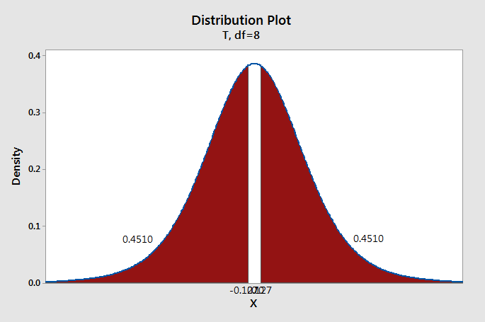
\(p=0.4510+0.4510=0.9020\)
We will compare our \(p\)-value from step 3 to a standard alpha level of 0.05.
Because \(p>\alpha\), we fail to reject the null hypothesis.
There is not sufficient evidence to state that scores on the two quizzes are different.
8.3.3 - Minitab: Paired Means Test
8.3.3 - Minitab: Paired Means TestThe steps for constructing a confidence interval or conducting a paired means \(t\) in Minitab are identical. The output that the procedure provides includes both the confidence interval and the \(p\)-value for determining statistical significance.
Minitab® – Conducting a Paired Means Test
Let's compare students' SAT-Math scores to their SAT-Verbal scores.
- Open the Minitab file: class_survey.mpx
- Select Stat > Basic Statistics > Paired t
- Select Each sample is in a column since we have the data in the worksheet
- Double click the variable SATM in the box on the left to insert the variable into the Sample 1 box
- Double click the variable SATV in the box on the left to insert the variable into the Sample 2 box
- Click OK
This should result in the following output:
Paired t: SATM, SATV
| Sample | N | Mean | StDev | SE Mean |
|---|---|---|---|---|
| SATM | 215 | 599.81 | 84.70 | 5.78 |
| SATV | 215 | 580.33 | 82.44 | 5.62 |
| Mean | StDev | SE Mean | 95% CI for \(\mu_d\) |
|---|---|---|---|
| 19.49 | 89.81 | 6.12 | (7.42, 31.56) |
\(\mu\)_difference: population mean of (SATM - SATV)
| Null hypothesis | H0: \(\mu\)_difference = 0 |
|---|---|
| Alternative hypothesis | H1: \(\mu\)_difference ≠ 0 |
| T-Value | P-Value |
|---|---|
| 3.18 | 0.002 |
On the next page, the five-step hypothesis testing procedure is used to interpret this output.
8.3.3.1 - Example: SAT Scores
8.3.3.1 - Example: SAT ScoresExample: SAT Scores
This example uses the dataset from Lesson 8.3.3 to walk through the five-step hypothesis testing procedure using the Minitab output.
Research question: Do students score differently on the SAT-Math and SAT-Verbal tests?
Because the sample size is large (\(n \ge 30\)), the t distribution may be used to approximate the sampling distribution.
\(H_{0}:\mu_d=0\)
\(H_{a}:\mu_d \ne 0\)
| Null hypothesis | H0: \(\mu_d\) = 0 |
|---|---|
| Alternative hypothesis | H1: \(\mu_d\) ≠ 0 |
| T-Value | P-Value |
|---|---|
| 3.18 | 0.002 |
The t test statistic is 3.18.
From the output, the p value is 0.002
\(p\leq .05\), therefore our decision is to reject the null hypothesis
There is evidence that in the population, on average, students' SAT-Math and their SAT-Verbal scores are different.
8.3.3.2 - Example: Marriage Age (Summarized Data)
8.3.3.2 - Example: Marriage Age (Summarized Data)In a sample of 105 married heterosexual couples, the average age difference (husband's age - wife's age) was 2.829 years with a standard deviation of 4.995 years. These summary statistics were taken from a data set from the Lock5 textbook. Is there evidence that, on average, in the population, husbands tend to be older than their wives?
First we need to check our assumptions. In this case the sample size is greater than 30 so we can use the t-distribution.
We know n = 105, \(\mu_{\text{husband's age}}-\mu_{\text{wife's age}}=2.829\), and \(s=4.995\). Since we want to know if the husbands are older than their wives then our difference in ages would be positive. So our alternative hypothesis is \(H_a\colon \gt 0\).
To complete this using Minitab...
- Select Stat > Basic Statistics > Paired t
- Select Summarized data (differences)
- For sample size enter 105, enter 2.829 for sample mean and 4.995 for standard deviation.
- Select Options
- The Hypothesized difference should be 0. (or 0.0)
- Select Difference > hypothesized difference for the Alternative hypothesis
- Click OK and OK
Estimation for Paired Difference
| Mean | StDev | SE Mean | 95% CI for \(\mu_d\) |
|---|---|---|---|
| 105 | 2.829 | 4.995 | (1.862, 3.796 |
\(\mu\)_difference: population mean of (Sample 1 - Sample 2)
Test
| Null hypothesis | H0: \(\mu\)_difference = 0 |
|---|---|
| Alternative hypothesis | H1: \(\mu\)_difference ≠ 0 |
| T-Value | P-Value |
|---|---|
| 5.80 | 0.000 |
Interpret the results
Because the sample size is large (\(n \ge 30\)), the t distribution may be used to approximate the sampling distribution.
\(H_{0}:\mu_d=0\)
\(H_{a}:\mu_d \gt 0\)
| Null hypothesis | H0: \(\mu_d\) = 0 |
|---|---|
| Alternative hypothesis | H1: \(\mu_d\) > 0 |
| T-Value | P-Value |
|---|---|
| 5.80 | 0.000 |
The t test statistic is 5.80.
From the output, the p value is 0.000
\(p\leq .05\), therefore our decision is to reject the null hypothesis
There is evidence that in the population, on average, the husband's age in heterosexual couples is greater than the wife's age.
8.4 - Lesson 8 Summary
8.4 - Lesson 8 SummaryObjectives
- Identify situations in which the z or t distributions may be used to approximate a sampling distribution
- Construct a confidence interval to estimate a population proportion, mean, or difference in paired means by hand given summary data
- Construct a confidence interval to estimate a population proportion, mean, or difference in paired means using Minitab given summary or raw data
- Determine the necessary minimum sample size to construct a confidence interval for a single proportion or single mean with a given level of confidence and margin of error
- Conduct a hypothesis test using the appropriate common distribution for a single proportion, single mean, and paired means by hand given summary data
- Conduct a hypothesis test using the appropriate common distribution for a single proportion, single mean, and paired means using Minitab given summary or raw data
In this lesson you learned how to construct confidence intervals and conduct hypothesis tests for one proportion, one mean, and paired means using the \(z\) and \(t\) distributions. These procedures are sometimes referred to as "traditional" methods, in contrast to the bootstrapping and randomization procedures that we learned earlier in the course which are "simulation-based inference" methods.
The table below summarizes the procedures covered in this lesson. Note the similarities between all of the confidence interval formulas and all of the test statistic formulas. These all follow the same general format.
| Procedure | Assumptions | Standard Error | Confidence Interval | Test Statistic |
|---|---|---|---|---|
| One Proportion \(z\) |
Confidence interval: At least 10 successes and 10 failures in the sample Hypothesis test: \(n p_0 \ge 10\) and \(n (1-p_0) \ge 10\) |
\(\sqrt{\dfrac{p(1-p)}{n}}\) | \(\widehat{p} \pm z^{*} \left ( \sqrt{\dfrac{\hat{p} (1-\hat{p})}{n}} \right) \) | \(z=\dfrac{\widehat{p}- p_0 }{\sqrt{\frac{p_0 (1- p_0)}{n}}}\) |
| One Mean \(t\) |
Sample size is at least 30 OR population is normally distributed Population standard deviation is unknown* |
\(\dfrac{\sigma}{\sqrt n}\) | \(\overline{x} \pm t^{*} \dfrac{s}{\sqrt{n}}\) | \(t=\dfrac{\overline{x}-\mu_0}{\frac{s}{\sqrt{n}}} \) |
| Paired Means \(t\) | Sample size is at least 30 OR differences are normally distributed in the population | \(\dfrac{\sigma_d}{\sqrt n}\) | \(\overline{x}_d \pm t^* \left(\dfrac{s_d}{\sqrt{n}}\right) \) | \(t=\dfrac{\bar{x}_d-\mu_0}{\frac{s_d}{\sqrt{n}}}\) |
* If the population standard deviation is known, then the sampling distribution may be approximated by a \(z\) distribution.
This lesson may be overwhelming if you are trying to memorize all of the formulas that were introduced. Luckily, doing so is unnecessary. You should focus on seeing the similarities between all of the procedures. For one sample mean, one sample proportion, paired means, two independent means, and two independent proportions, the following general formulas can be applied
- General Form of a Confidence Interval
- \(sample\ statistic\pm(multiplier)\ (standard\ error)\)
- General Form of a Test Statistic
- \(test\;statistic=\dfrac{sample\;statistic-null\;parameter}{standard\;error}\)
Also, when given raw data, use Minitab. It is much more efficient than performing calculations by hand.