8.2.3.1 - One Sample Mean t Test, Formulas

Five Step Hypothesis Testing Procedure

1. Check assumptions and write hypotheses

Data must be quantitative. In order to use the t distribution to approximate the sampling distribution either the sample size must be large ($\ge\ 30$) or the population must be known to be normally distributed. The possible combinations of null and alternative hypotheses are:

Research Question	Is the mean different from $ \mu_{0} $?	Is the mean greater than $\mu_{0}$?	Is the mean less than $\mu_{0}$?
Null Hypothesis, $H_{0}$	$\mu=\mu_{0} $	$\mu=\mu_{0} $	$\mu=\mu_{0} $
Alternative Hypothesis, $H_{a}$	$\mu\neq \mu_{0} $	$\mu> \mu_{0} $	$\mu<\mu_{0} $
Type of Hypothesis Test	Two-tailed, non-directional	Right-tailed, directional	Left-tailed, directional

where $ \mu_{0} $ is the hypothesized population mean.

2. Calculate the test statistic

For the test of one group mean we will be using a $t$ test statistic:

Test Statistic: One Group Mean

$t=\dfrac{\overline{x}-\mu_0}{\frac{s}{\sqrt{n}}}$

$\overline{x}$ = sample mean
$\mu_{0}$ = hypothesized population mean
$s$ = sample standard deviation
$n$ = sample size

Note that structure of this formula is similar to the general formula for a test statistic:

$\dfrac{sample\;statistic-null\;value}{standard\;error}$

3. Determine the p-value

When testing hypotheses about a mean or mean difference, a $t$ distribution is used to find the $p$-value. These $t$ distributions are indexed by a quantity called degrees of freedom, calculated as $df = n – 1$ for the situation involving a test of one mean or test of mean difference. The $p$-value can be found using Minitab.

4. Make a decision

If $p \leq \alpha$ reject the null hypothesis.

If $p>\alpha$ fail to reject the null hypothesis.

5. State a "real world" conclusion

Based on your decision in Step 4, write a conclusion in terms of the original research question.

The new few pages will walk you through examples before giving you the opportunity to do two on your own.

8.2.3.1.1 - Video Example: Book Costs

Research question: Does the average Penn State student spend more than \$300 each semester on textbooks?

In a sample of 226 Penn State students, the mean cost of a student’s textbooks was \$344 with a standard deviation of \$106.

8.2.3.1.2 : Example: Pulse Rate

A research study measured the pulse rates of 57 college men and found a mean pulse rate of 70.4211 beats per minute with a standard deviation of 9.9480 beats per minute. Researchers want to know if the mean pulse rate for all college men is different from the current standard of 72 beats per minute.

1. Check assumptions and write hypotheses

Pulse rates are quantitative. The sampling distribution will be approximately normally distributed because $n \ge 30$.

This is a two-tailed test because we want to know if the mean pulse rate is different from 72.

$H_{0}:\mu=72 $
$H_{a}: \mu\neq 72 $

2. Calculate the test statistic

Test Statistic: One Group Mean

$t=\dfrac{\overline{x}-\mu_0}{\dfrac{s}{\sqrt{n}}}$

$\overline{x}$ = sample mean
$\mu_{0}$ = hypothesized population mean
$s$ = sample standard deviation
$n$ = sample size

$t=\dfrac{\overline{x}-\mu_0}{\dfrac{s}{\sqrt{n}}}=\dfrac{70.4211-72}{\dfrac{9.9480}{\sqrt{57}}}=-1.198$

Our $t$ test statistic is -1.198

3. Determine the p-value

$df=n-1=57-1=56$

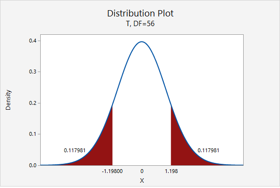
Distribution Plot of Density vs X - T, DF=56

$p=0.117981+0.117981=0.235962$

Given that the null hypothesis is true and $\mu=72$, the probability of taking a random sample of $n=57$ and finding a sample mean this or more extremely different is 0.235962. This is our p-value.

4. Make a decision

$p>.05$, therefore we fail to reject the null hypothesis.

5. State a "real world" conclusion

There is not sufficient evidence to state that the mean pulse of college men is different from 72.

8.2.3.1.3 - Example: Coffee

In the population of Americans who drink coffee, the average daily consumption is 3 cups per day. A university wants to know if their students tend to drink more coffee than the national average. They ask a random sample of 50 students how many cups of coffee they drink each day and found $\overline{x}=3.8$ and $s=1.5$. Do they have evidence that their students drink more than the national average?

1. Check assumption and write hypotheses

Amount of coffee consumed is a quantitative variable. We are given that random sampling methods were employed. Because $n \ge 30$, we can approximate the sampling distribution using a t distribution.

This is a right-tailed test because we want to know if the mean in the sample is greater than the national average.

$H_{0}:\mu= 3$
$H_{a}:\mu>3$

2. Calculate the test statistic

Test Statistic: One Group Mean

$t=\dfrac{\overline{x}-\mu_0}{\dfrac{s}{\sqrt{n}}}$

$\overline{x}$ = sample mean
$\mu_{0}$ = hypothesized population mean
$s$ = sample standard deviation
$n$ = sample size

$t=\dfrac{\overline{x}-\mu_0}{\dfrac{s}{\sqrt{n}}}=\dfrac{3.8-3}{\dfrac{1.5}{\sqrt{50}}}=3.771$

Our $t$ test statistic is 3.771

3. Determine the p-value

$df=n-1=50-1=49$

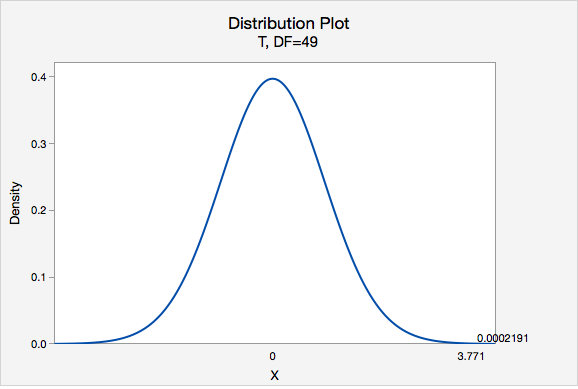
Distribution Plot of Density vs X - T, DF=49

Using Minitab, we can find that $P(t > 3.771) =0.0002191$

p-value = 0.0002191

If $\mu=3$, then the probability of taking a random sample of $n=50$ and finding $\overline{x} \geq 3$ is 0.0002191

4. Make a decision

$p\leq.05$, therefore we reject the null hypothesis.

5. State a "real world" conclusion

There is evidence to state the mean number of coffees consumed in the population of all students at this university is greater than 3.

8.2.3.1.4 - Example: Transportation Costs

According to CNN, in 2011, the average American spent \$16,803 on housing. A suburban community wants to know if their residents spent less than this national average. In a survey of 30 randomly selected residents, they found that they spent an annual average of \$15,800 with a standard deviation of \$2,600.

1. Check assumptions and write hypotheses

Housing costs are quantitative. Because $n \ge 30$, the sampling distribution can be approximated using the $t$ distribution.

This is a left-tailed test because we want to know if residents of this community spent less than the national average.

$H_{0}:\mu=16803$
$H_{a}:\mu<16803$

2. Calculate the test statistic

Test Statistic: One Group Mean

$t=\dfrac{\overline{x}-\mu_0}{\dfrac{s}{\sqrt{n}}}$

$\overline{x}$ = sample mean
$\mu_{0}$ = hypothesized population mean
$s$ = sample standard deviation
$n$ = sample size

$t=\dfrac{\overline{x}-\mu_0}{\dfrac{s}{\sqrt{n}}}=\dfrac{15800-16803}{\dfrac{2600}{\sqrt{30}}}=-2.113$

Our t test statistics is -2.113

3. Determine the p-value

$df=n-1=30-1=29$

This is a left-tailed test so we want to know the probability of $t < -2.113$

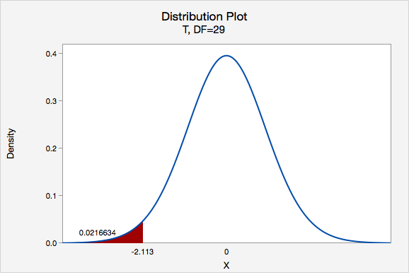
Distribution Plot of Density vs X - T, DF=29

Using Minitab we can find that $p=0.0216634$

4. Make a decision

$p\leq .05$, therefore we reject the null hypothesis.

5. State a "real world" conclusion

There is evidence to state that on average residents of this community spent less than the national average on housing in 2011.

Research Question	Is the mean different from \( \mu_{0} \)?	Is the mean greater than \(\mu_{0}\)?	Is the mean less than \(\mu_{0}\)?
Null Hypothesis, \(H_{0}\)	\(\mu=\mu_{0} \)	\(\mu=\mu_{0} \)	\(\mu=\mu_{0} \)
Alternative Hypothesis, \(H_{a}\)	\(\mu\neq \mu_{0} \)	\(\mu> \mu_{0} \)	\(\mu<\mu_{0} \)
Type of Hypothesis Test	Two-tailed, non-directional	Right-tailed, directional	Left-tailed, directional

^[1]	Link
↥	Has Tooltip/Popover
	Toggleable Visibility