10: One-Way ANOVA
10: One-Way ANOVAObjectives
- Explain why it is not appropriate to conduct multiple independent t tests to compare the means of more than two independent groups
- Use Minitab to construct a probability plot for an F distribution
- Use Minitab to perform a one-way between groups ANOVA with Tukey's pairwise comparisons
- Interpret the results of a one-way between groups ANOVA
- Interpret the results of Tukey's pairwise comparisons
In previous lessons you learned how to compare the means of two independent groups. In this lesson, we will learn how to compare the means of more than two independent groups. This procedure is known as a one-way between groups analysis of variance, or more often as a "one-way ANOVA."
Why not multiple independent t-tests?
A frequently asked question is, "why not just perform multiple two independent samples \(t\) tests?" If you were to perform multiple independent \(t\) tests instead of a one-way between groups ANOVA you would need to perform more tests. For \(k\) independent groups there are \(\frac{k(k-1)}{2}\) possible pairs. If you had 5 independent groups, that would equal \(\frac{5(5-1)}{2}=10\) independent t tests! And, those 10 independent t tests would not give you information about the independent variable overall. Most importantly, multiple \(t\) tests would lead to a greater chance of making a Type I error. By using an ANOVA, you avoid inflating \(\alpha\) and you avoid increasing the likelihood of a Type I error.
10.1 - Introduction to the F Distribution
10.1 - Introduction to the F DistributionOne-way ANOVAs, along with a number of other statistical tests, use the F distribution. Earlier in this course you learned about the \(z\) and \(t\) distributions. You computed \(z\) and \(t\) test statistics and used those values to look up p-values using statistical software. Similarly, in this lesson you are going to compute F test statistics. The F test statistic can be used to determine the p-value for a one-way ANOVA.
The video below gives a brief introduction to the F distribution and walks you through two examples of using Minitab to find the p-values for given F test statistics. The steps for creating a distribution plot to find the area under the F distribution are the same as the steps for finding the area under the \(z\) or \(t\) distribution. For the F distribution we will always be looking for a right-tailed probability. Later in this lesson we will see that this area is the p-value.
The F distribution has two different degrees of freedom: between groups and within groups. Minitab will call these the numerator and denominator degrees of freedom, respectively. Within groups is also referred to as error.
- Between Groups (Numerator) Degrees of Freedom
-
\(df_{between}=k-1\)
-
\(k\) = number of groups
- Within Groups (Denominator, Error) Degrees of Freedom
-
\(df_{within}=n-k\)
-
\(n\) = total sample size with all groups combined
\(k\) = number of groups
Minitab® – Creating an F Distribution
Scenario: An F test statistic of 2.57 is computed with 3 and 246 degrees of freedom. What is the p-value for this test?
We can create a distribution plot. Our distribution is the F distribution. The numerator df (\(df_1\)) is 3 and the denominator df (\(df_2\)) is 246. We want to shade the area in the right tail. Our “X Value” is 2.57.
- Open Minitab
- Select Graph > Probability Distribution Plot > View Probability
- Change the Distribution to F
- Fill in the Numerator degrees of freedom with 3 and the Denominator degrees of freedom with 246
- Select the Options button
- Select A specified x value
- Use the default Right tail
- For the X value enter 2.57
- OK and OK
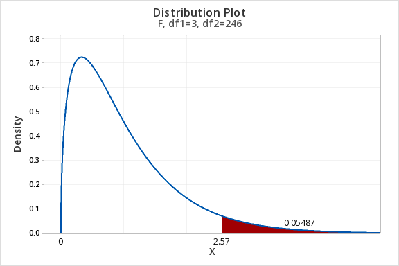
The area beyond an F-value of 2.57 with 3 and 246 degrees of freedom is 0.05487. The p-value for this F test is 0.05487.
Note: When you conduct an ANOVA in Minitab, the software will compute this p-value for you.
10.2 - Hypothesis Testing
10.2 - Hypothesis TestingA one-way between groups ANOVA is used to compare the means of more than two independent groups. A one-way between groups ANOVA comparing just two groups will give you the same results at the independent \(t\) test that you conducted in Lesson 8. We will use the five step hypothesis testing procedure again in this lesson.
The assumptions for a one-way between groups ANOVA are:
- Samples are independent
- The response variable is approximately normally distributed for each group or all group sample sizes are at least 30
- The population variances are equal across responses for the group levels (if the largest sample standard deviation divided by the smallest sample standard deviation is not greater than two, then assume that the population variances are equal)
Given that you are comparing \(k\) independent groups, the null and alternative hypotheses are:
\(H_{0}: \mu_1 = \mu_2 = \cdots = \mu_k\)
\(H_{a}:\) Not all \(\mu_\cdot\) are equal
In other words, the null hypothesis is that at all of the groups' population means are equal. The alternative is that they are not all equal; there are at least two population means that are not equal to one another.
ANOVA uses an F test statistic. Hand calculations for ANOVAs require many steps. In this class, you will be working primarily with Minitab outputs.
Conceptually, the F statistic is a ratio: \(F=\frac{Between\;groups\;variability}{Within\;groups\;variability}\). Numerically this translates to \(F=\frac{MS_{Between}}{MS_{Within}}\). In other words how much do individuals in different groups vary from one another over how much to individuals within groups vary from one another.
Statistical software will compute the F ratio for you and produce what is known as an ANOVA source table. The ANOVA source table will give you information about the variability between groups and within groups. The table below gives you all of the formulas, but you will not be responsible for performing these calculations by hand. Minitab will do all of these calculations for you and provide you with the full ANOVA source table.
| Source | df | SS | MS | F | p |
|---|---|---|---|---|---|
| Between Groups (Factor) | \(k-1\) | \(\sum_{k}n_k(\overline{x}_k-\overline{x}_\cdot)^2\) | \(\dfrac{SS_{Between}}{df_{Between}}\) | \(\dfrac{MS_{Between}}{MS_{Within}}\) | Area to the right of Fk-1, n-k |
| Within Groups (Error) | \(n-k\) | \(\sum_k \sum_i(x_{ik}-\overline{x}_k)^2\) | \(\dfrac{SS_{Within}}{df_{Within}}\) | ||
| Total | \(n-1\) | \(\sum_k \sum_i(x_{ik}-\overline{x}_\cdot)^2\) |
| \(k\) | Number of groups |
| \(n\) | Total sample size (all groups combined) |
| \(n_k\) | Sample size of group \(k\) |
| \(\overline{x}_k\) | Sample mean of group \(k\) |
| \(\overline{x}_\cdot\) | Grand mean (i.e., mean for all groups combined) |
| SS | Sum of squares |
| MS | Mean square |
| df | Degrees of freedom |
| F | F-ratio (the test statistic) |
Some of the terms in the table above should look familiar, while others will be new to you. The sum of squares that appears in the ANOVA source table is similar to the sum of squares that you computed in Lesson 2 when computing variance and standard deviation. Recall, the sum of squares is the squared difference between each score and the mean. Here, there are three different sum of squares each measuring a different type of variability.
The ANOVA source table also has three different degrees of freedom: \(df_{between}\), \(df_{within}\), and \(df_{total}\). If you were to look up an F value using statistical software you would need to know two of these degrees of freedom: \(df_1 = df_{between}\) and \(df_2=df_{within}\).
When performing an ANOVA using statistical software, you will be given the p-value in the ANOVA source table. If performing an ANOVA by hand, you would use the F distribution. Similar to the t distribution, the F distribution varies depending on degrees of freedom.
If \(p \leq \alpha\) reject the null hypothesis. If \(p>\alpha\) fail to reject the null hypothesis.
Based on your decision in Step 4, write a conclusion in terms of the original research question.
10.3 - Pairwise Comparisons
10.3 - Pairwise ComparisonsWhile the results of a one-way between groups ANOVA will tell you if there is what is known as a main effect of the explanatory variable, the initial results will not tell you which groups are different from one another. In order to determine which groups are different from one another, a post-hoc test is needed. Post-hoc tests are conducted after an ANOVA to determine which groups differ from one another. There are many different post-hoc analyses that could be performed following an ANOVA. Here, we will learn about one of the most common tests known as Tukey's Honestly Significant Differences (HSD) Test.
Most statistical software, including Minitab, will compute Tukey's pairwise comparisons for you. This specific post-hoc test makes all possible pairwise comparisons. In this class we will be relying on statistical software to perform these analyses, if you are interested in seeing how the calculations are performed, this information is contained in the notes for STAT 502: Analysis of Variance and Design of Experiments. This analysis takes into account the fact that multiple tests are being performed and makes the necessary adjustments to ensure that Type I error is not inflated.
In the examples later in this lesson you will see a number of Tukey post-hoc tests. Next, you will also learn how to obtain these results using Minitab.
For each pairwise comparison, \(H_0: \mu_i - \mu_j=0\) and \(H_a: \mu_i - \mu_j \ne 0\).
10.4 - Minitab: One-Way ANOVA
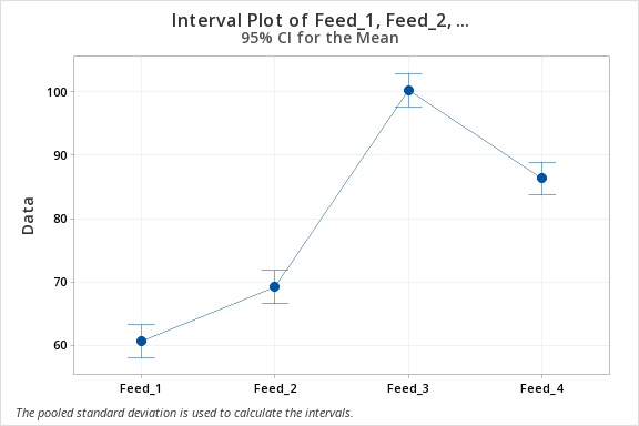
10.4 - Minitab: One-Way ANOVAIn one research study, 20 young pigs are assigned at random among 4 experimental groups. Each group is fed a different diet. (This design is a completely randomized design.) The data are the pigs' weights in kg after being raised on these diets for 10 months. We wish to determine if there are any differences in mean pig weights for the 4 diets.
- \(H_0: \mu_1 = \mu_2 = \mu_3 = \mu_4\)
- \(H_a:\) Not all \(\mu\) are equal
| Feed_1 | Feed_2 | Feed_3 | Feed_4 |
|---|---|---|---|
| 60.8 | 68.3 | 102.6 | 87.9 |
| 57.1 | 67.7 | 102.2 | 84.7 |
| 65.0 | 74.0 | 100.5 | 83.2 |
| 58.7 | 66.3 | 97.5 | 85.8 |
| 61.8 | 69.9 | 98.9 | 90.3 |
Contained in the Minitab file: ANOVA_ex.mpx
Note that in this file the data were entered so that each group is in its own column. In other words, the responses are in a separate column for each factor level. In later examples, you will see that Minitab will also conduct a one-way ANOVA if the responses are all in one column with the factor codes in another column.
Minitab® – One-Way ANOVA
To perform an Analysis of Variance (ANOVA) test in Minitab:
- Open the Minitab file: ANOVA_ex.mpx
- From the menu bar, select Stat > ANOVA > One-Way.
- Click the drop-down menu and select 'Responses are in a separate column for each factor level'.
- Enter the variables Feed_1, Feed_2, Feed_3, and Feed_4 to insert them into the Responses box.
- Choose the Comparisons button and check the box next to Tukey. Under Results also select Tests.
- OK and OK
The result should be the following output:
Method
| Null hypothesis | All means are equal |
|---|---|
| Alternative hypothesis | At least one mean is different |
| Significance level | \(\alpha=0.05\) |
Equal variances were assumed for the analysis
Factor Information
| Factor | Levels | Values |
|---|---|---|
| Factor | 4 | Feed_1, Feed_2, Feed_3, Feed_4 |
Analysis of Variance
| Source | DF | Adj SS | Adj MS | F-Value | P-Value |
|---|---|---|---|---|---|
| Factor | 3 | 4703.2 | 1567.73 | 206.72 | 0.000 |
| Error | 16 | 121.3 | 7.58 | ||
| Total | 19 | 4824.5 |
Model Summary
| S | R-sq | R-sq(adj) | R-sq(pred) |
|---|---|---|---|
| 2.75386 | 97.48% | 97.01% | 96.07% |
Means
| Factor | N | Mean | StDev | 95% CI |
|---|---|---|---|---|
| Feed_1 | 5 | 60.68 | 3.03 | (58.07, 63.29) |
| Feed_2 | 5 | 69.24 | 2.96 | (66.63, 71.85) |
| Feed_3 | 5 | 100.340 | 2.164 | (97.729, 102.951) |
| Feed_4 | 5 | 86.38 | 2.78 | (83.77, 88.99) |
Pooled StDev = 2.75386
Grouping Information Using the Tukey Method and 95% Confidence
| Factor | N | Mean | Grouping | |||
|---|---|---|---|---|---|---|
| Feed_3 | 5 | 100.34 | A | |||
| Feed_4 | 5 | 86.38 | B | |||
| Feed_2 | 5 | 69.24 | C | |||
| Feed_1 | 5 | 60.68 | D | |||
Means that do not share a letter are significantly different.
| Difference of Levels |
Difference of Means |
SE of Difference |
95% CI | T-Value | Adjusted P-Value |
|---|---|---|---|---|---|
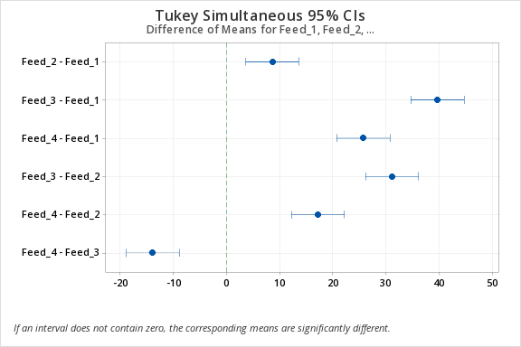
| Feed_2 - Feed_1 | 8.56 | 1.74 | (3.57, 13.55) | 4.91 | 0.001 |
| Feed_3 - Feed_1 | 39.66 | 1.74 | (34.67, 44.65) | 22.77 | 0.000 |
| Feed_4 - Feed_1 | 25.70 | 1.74 | (20.71, 30.69) | 14.76 | 0.000 |
| Feed_3 - Feed_2 | 31.10 | 1.74 | (26.11, 36.09) | 17.86 | 0.000 |
| Feed_4 - Feed_2 | 17.14 | 1.74 | (12.15, 22.13) | 9.84 | 0.000 |
| Feed_4 - Feed_3 | -13.96 | 1.74 | (-18.95, -8.97) | -8.02 | 0.000 |
Tukey Simultaneous Tests for Differences of Means
Individual confidence level = 98.87%
10.5 - Example: SAT-Math Scores by Award Preference
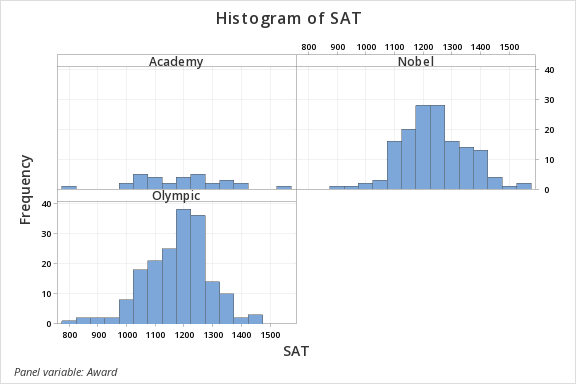
10.5 - Example: SAT-Math Scores by Award PreferenceIn this example, we are comparing the SAT scores of students who said that they would prefer to win an Academy Award, a Nobel Prize, or an Olympic gold medal.
The example uses the StudentSurvey dataset provided by the Lock5 textbook.
Let's apply the five-step hypothesis testing process to this example.
The assumptions for a one-way between-groups ANOVA are:
Assumption: Samples are independent: Each student selected either Olympic, Academy, or Nobel. Each student is in only one group and those groups are in no way matched or paired. This assumption is met.
Assumption: The response variable is approximately normally distributed for each group or all group sample sizes are at least 30: To check this we can construct a histogram with groups in Minitab. These plots show that the distributions are all approximately normal.
Assumption: The population variances are equal across responses for the group levels (if the largest sample standard deviation divided by the smallest sample standard deviation is not greater than two, then assume that the population variances are equal). Again we can use Minitab to look at the standard deviations across the groups. The largest standard deviation is 151.3 and the smallest is 114.1 for a ratio of 1.33 which is less than 2. So this assumption is met.
Statistics
Award | N | N* | Mean | SE Mean | StDev | Minimum | Q1 | Median | Q3 | Maximum |
|---|---|---|---|---|---|---|---|---|---|---|
Academy | 31 | 0 | 1191.0 | 27.2 | 151.3 | 820.0 | 1070.0 | 1200.0 | 1300.0 | 1530.0 |
Nobel | 149 | 0 | 1239.1 | 9.38 | 114.5 | 920.0 | 1160.0 | 1230.0 | 1310.0 | 1550.0 |
Olympic | 182 | 0 | 1176.7 | 8.46 | 114.1 | 800.0 | 1100.0 | 1190.0 | 1250.0 | 1470.0 |
Use Minitab to run a one-way ANOVA with the Minitab file: StudentSurvey.mpx
The following will describe the output within the context of the five-step hypothesis testing process.
Given that you are comparing \(k\) independent groups, the null and alternative hypotheses are:
Method
Null hypothesis | All means are equal |
|---|---|
Alternative hypothesis | At least one mean is different |
Significance level | \(\alpha=0.05\) |
Equal variances were assumed for the analysis
You should get the following output:
Factor Information
Factor | Levels | Values |
|---|---|---|
Award | 3 | Academy, Nobel, Olympic |
The factor information tells us that our factor is the Award.
Analysis of Variance
Source | DF | Adj SS | Adj MS | F-Value | P-Value |
|---|---|---|---|---|---|
Award | 2 | 323269 | 162134 | 11.67 | 0.000 |
Error | 359 | 4986078 | 13889 | ||
Total | 361 | 5310347 |
The analysis of variance table is also known as our ANOVA source table. The source of the Award is our between-groups variation so the DF K -1 or 3-1 = 2. Error is our within-groups variation so the degrees of freedom are n - K or 362-3 = 359. The 'Adj' stands for adjusted. For a one-way ANOVA, nothing is being adjusted. The F-value is our F-test statistic, which in this case is 11.67 with a p-value of 0.000. The F value could be written as F (2, 359) = 11.67.
Means
Factor | N | Mean | StDev | 95% CI |
|---|---|---|---|---|
Academy | 31 | 1191.0 | 151.3 | (1149.3, 1232.6) |
Nobel | 149 | 1239.11 | 114.54 | (1220.13, 1258.10) |
Olympic | 182 | 1176.73 | 114.13 | (1159.55, 1193.91) |
Pooled StDev = 117.851
The Means table is just a table of descriptive statistics. The sample size, mean, and the standard deviation is presented for each group. The last column is an unadjusted 95% confidence interval. You should not refer to these confidence intervals since these do not take into account that there are three different groups and three different confidence intervals being computed at the same time. The confidence intervals that we're interested in come with our Tukey pairwise comparison.
need to know two of these degrees of freedom: \(df_1 = df_{between}\) and \(df_2=df_{within}\).
The p-value is 0.000 from the Minitab output.
\(p \leq \alpha\) so reject the null hypothesis.
We can conclude that the group means are not all equal.
Remember that ANOVA is just an omnibus test. It only tells us there is a difference somewhere. To determine where the differences are you would have to look at the Tukey pairwise comparison output.
Grouping Information Using the Tukey Method and 95% Confidence
Award | N | Mean | Grouping | |
|---|---|---|---|---|
Nobel | 149 | 1239.11 | A | |
Academy | 31 | 1190.97 | A | B |
Olympic | 182 | 1176.73 | B | |
Means that do not share a letter are significantly different.
In the grouping table, Nobel and Olympic do not share a grouping letter. The means of these two groups are significantly different. Both the Nobel and Academy belong to Group A and both Academy and Olympic belong to Group B. These pairs are not significantly different.
Tukey Simultaneous Tests for Differences of Means
Difference of Levels | Difference | SE of | 95% CI | T-Value | Adjusted |
|---|---|---|---|---|---|
Nobel - Academy | 48.1 | 23.3 | (-6.3, 102.6) | 2.07 | 0.096 |
Olympic - Academy | -14.2 | 22.9 | (-67.8, 39.4) | -0.62 | 0.808 |
Olympic - Nobel | -62.4 | 13.0 | (-92.9, -31.9) | -4.79 | 0.000 |
Individual confidence level = 98.87%
The Tukey Simultaneous Tests table provides the adjusted 95% confidence intervals. These are the confidence intervals and p-values you should be looking at when you're making pairwise comparisons. These are adjusted to take into account that there are three different pairwise tests being performed simultaneously. To determine which groups are statistically significant we can look at the adjusted p-value. In this case, the only p-value less than 0.05 is the Olympic - Nobel pairwise comparison. The means of the Olympic and Nobel group are significantly different.
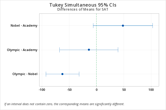
In the Tukey Simultaneous 95% CI graph any interval not containing zero indicates a statistically significant difference. In this case, we see that the Olympic - Nobel group does not contain zero so this pairing has a statistically significant difference.
10.6 - Example: Exam Grade by Professor
10.6 - Example: Exam Grade by ProfessorScenario
Three professors were each teaching one section of a course. They all gave the same final exam and they want to know if there are any differences between their sections’ mean scores.
\(H_0:\mu_1=\mu_2=\mu_3\)
\(H_a: Not\;all\;\mu\;are\;equal\)
Means
| Instructor | N | Mean | StDev | 95% CI |
|---|---|---|---|---|
| Dr. Al | 60 | 68.367 | 17.719 | (63.977, 72.756) |
| Dr. Oh | 87 | 71.448 | 16.702 | (67.803, 75.094) |
| Dr. Pa | 98 | 67.939 | 17.465 | (64.504, 71.373) |
Pooled StDev = 17.2609
The standard deviations for all three classes are all similar.
- Open the Minitab file: ANOVA_Exam_Profs.mpx
- Using Minitab: Stat > ANOVA > One-Way
The result is the following ANOVA source table:
Analysis of Variance
| Source | DF | Adj SS | Adj MS | F-Value | P-Value |
|---|---|---|---|---|---|
| Instructor | 2 | 635.3 | 317.7 | 1.07 | 0.346 |
| Error | 242 | 72101.1 | 297.9 | ||
| Total | 244 | 72736.4 |
F (2, 242) = 1.07
From our ANOVA source table, p = .346
Because \(p > \alpha\), we fail to reject the null hypothesis.
There is not enough evidence to conclude that the mean scores from the three different professors’ sections are different.
Tukey Pairwise Comparisons
There is some debate as to whether pairwise comparisons are appropriate when the overall one-way ANOVA is not statistically significant. Some argue that if the overall ANOVA is not significant then pairwise comparisons are not necessary. Others argue that if the pairwise comparisons were planned before the ANOVA was conducted (i.e., "a priori") then they are appropriate.
The results of our Tukey pairwise comparisons were as follows:
Grouping Information Using the Tukey Method and 95% Confidence
| Instructor | N | Mean | Grouping |
|---|---|---|---|
| Dr. Oh | 87 | 71.448 | A |
| Dr. Al | 60 | 68.367 | A |
| Dr. Pa | 98 | 67.939 | A |
Means that do not share a letter are significantly different.
Tukey Simultaneous Tests for Differences of Means
| Difference of Levels | Difference of Means | SE of Difference | 95% CI | T-Value | Adjusted P-Value |
|---|---|---|---|---|---|
| Dr. Oh-Dr. Al | 3.08 | 2.90 | (-3.70, 9.86) | 1.06 | 0.537 |
| Dr. Pa-Dr. Al | -0.43 | 2.83 | (-7.05, 6.19) | -0.15 | 0.987 |
| Dr. Pa-Dr. Oh | -3.51 | 2.54 | (-9.46, 2.44) | -1.38 | 0.351 |
Individual confidence level = 97.99%
Looking at the first table, all three instructors are in group A. Means that share a letter are not significantly different from one another (i.e., they are in the same group). Because all three instructors share the letter A, there are no significantly different pairs of instructors.
We could also look at the second table which gives us the t-test statistic and adjusted p-value for each possible pairwise comparison. This p-value is adjusted to take into account that multiple tests are being conducted. You can compare these p-values to the standard alpha level of .05. All p-values are greater than .05, therefore no pairs are significantly different from one another.
10.7 - Lesson 10 Summary
10.7 - Lesson 10 SummaryObjectives
- Explain why it is not appropriate to conduct multiple independent t tests to compare the means of more than two independent groups
- Use Minitab to construct a probability plot for an F distribution
- Use Minitab to perform a one-way between groups ANOVA with Tukey's pairwise comparisons
- Interpret the results of a one-way between groups ANOVA
- Interpret the results of Tukey's pairwise comparisons
In this lesson you learned how to compare the means of three or more groups using a one-way between groups ANOVA. A one-way between groups ANOVA is used instead of multiple independent \(t\) tests in order to avoid increasing the likelihood of committing a Type I error.
An ANOVA provides information about the explanatory variable overall, but not about differences between the different levels of that variable. In order to compare the different pairs we need to conduct a post-hoc analysis such as Tukey's HSD test.