11: Chi-Square Tests
11: Chi-Square TestsObjectives
- Construct a chi-square probability distribution plot in StatKey or Minitab
- Determine when a chi-square goodness-of-fit test and chi-square test of independence should be conducted
- Compute and interpret expected counts
- Conduct chi-square tests by hand and using Minitab
- Calculate and interpret relative risk
In this lesson we will learn how to compare the proportions of more than two independent groups and how to test for a relationship between two categorical variables. In this lesson you will also review risk and odds and learn about relative risk.
Before we begin, let's review the various classifications of variables from Lesson 1:
- Categorical
- Names or labels (i.e., categories) with no logical order or with a logical order but inconsistent differences between groups, also known as qualitative.
- Quantitative
- Numerical values with magnitudes that can be placed in a meaningful order with consistent intervals, also known as numerical.
In this lesson we will be examining methods for analyzing categorical variables.
11.1 - Reviews
11.1 - ReviewsIn this lesson you may need to use Minitab to construct frequency tables or two-way contingency tables. We'll start by reviewing these procedures. You will need to construct probability distribution plots for chi-square distributions. In earlier lessons we constructed probability distribution plots for z, t, and F distributions; the procedure is similar for a chi-square distribution. We will also review conditional probabilities and the term independence in this section.
11.1.1 - Frequency Table
11.1.1 - Frequency TableThe following example was first presented in Lesson 2.1.1.2.1.
It uses following data set (from College Board):
Minitab® – Frequency Tables
To create a frequency table in Minitab:
- Open the Minitab file: sat_data.mpx
- Select Stat > Tables > Tally Individual Variables
- Double click the variable Region in the box on the left to insert the variable into the Variable box
- Under Statistics, check Counts and Percents
- Click OK
This should result in the following frequency table:
Tally
| Region | Count | Percent |
|---|---|---|
| ENC | 5 | 9.80 |
| ESC | 4 | 7.84 |
| MA | 3 | 5.88 |
| MTN | 8 | 15.69 |
| NE | 6 | 11.76 |
| PAC | 5 | 9.80 |
| SA | 9 | 17.65 |
| WNC | 7 | 13.73 |
| WSC | 4 | 7.84 |
| N= | 51 |
11.1.2 - Two-Way Contingency Table
11.1.2 - Two-Way Contingency TableRecall from Lesson 2.1.2 that a two-way contingency table is a display of counts for two categorical variables in which the rows represented one variable and the columns represent a second variable. The starting point for analyzing the relationship between two categorical variables is to create a two-way contingency table. When one variable is obviously the explanatory variable, the convention is to use the explanatory variable to define the rows and the response variable to define the columns; this is not a hard and fast rule though.
Minitab® – Constructing a Two-Way Contingency Table
- Open the data set: class_survey.mpx
- Select Stat > Tables > Cross Tabulation and Chi-square
- Select Raw data (categorical variable) from the drop down menu
- Double click the variable Smoke Cigarettes in the box on the left to insert the variable into the Rows box
- Double click the variable Biological Sex in the box on the left to insert the variable into the Columns box
- Click OK
This should result in the two-way table below:
Rows: Smokes Cigaretes | Columns: Biological Sex
| Female | Male | All | |
|---|---|---|---|
| No | 120 | 89 | 209 |
| Yes | 7 | 10 | 17 |
| All | 127 | 99 | 226 |
| Cell Contents: Count | |||
11.1.3 - Probability Distribution Plots
11.1.3 - Probability Distribution PlotsIn previous lessons you have constructed probabilities distribution plots for normal distributions, binomial distributions, and \(t\) distributions. This week you will use the same procedure to construct a probability distribution plot for the chi-square distribution.
Minitab® – Constructing a Probability Distribution Plot
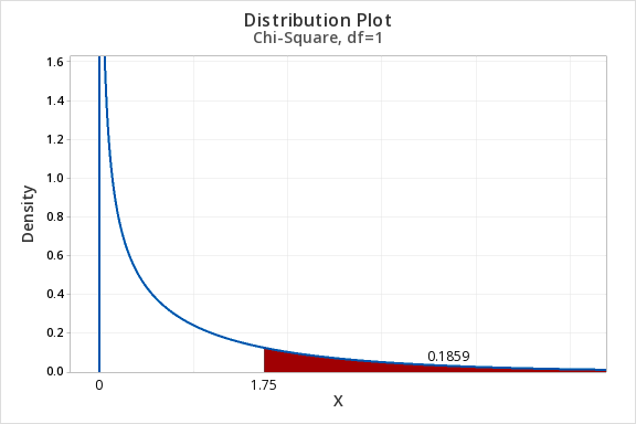
Chi-square tests of independence are always right-tailed tests. Let's find the area of a chi-square distribution with 1 degree of freedom to the right of \(\chi^2 = 1.75\). In other words, we're looking up the \(p\) value associated with a chi-square test statistic of 1.75.
- In Minitab, select Graph > Probability Distribution Plot > View Probability
- Choose Chi-Square for the Distribution
- For Distribution select Chi-Square
- For Degrees of freedom enter 1
- Select A specified X value
- Select Right tail
- For X value enter 1.75
- Select OK and OK
This should result in the following output:
Example: Area to the Right of Chi-Sq = 6.25, df=3
Construct a chi-square distribution with 3 degrees of freedom to find the area to the right of a chi-square value of 6.25.
- In Minitab, select Graph > Probability Distribution Plot > View Probability
- Choose Chi-Square for the Distribution
- For Distribution select Chi-Square
- For Degrees of freedom enter 3
- Select A specified X value
- Select Right tail
- For X value enter 6.25
- Select OK and OK
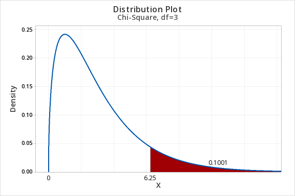
The area to the right of 6.25 in the chi-square distribution with 3 degrees of freedom is 0.1001.
11.1.4 - Conditional Probabilities and Independence
11.1.4 - Conditional Probabilities and IndependenceIn Lesson 2 you were introduced to conditional probabilities and independent events. These definitions are reviewed below along with some examples.
Recall that if events A and B are independent then \(P(A) = P(A \mid B)\). In other words, whether or not event B occurs does not change the probability of event A occurring.
- Conditional Probability
-
The probability of one event occurring given that it is known that a second event has occurred. This is communicated using the symbol \(\mid\) which is read as "given."
For example, \(P(A\mid B)\) is read as "Probability of A given B."
- Independent Events
- Unrelated events. The outcome of one event does not impact the outcome of the other event.
Example: Queens & Hearts
If a card is randomly drawn from a standard 52-card deck, the probability of the card being a queen is independent from the probability of the card being a heart. If I tell you that a randomly selected card is a queen, that does not change the likelihood of it being a heart, diamond, club, or spade.
Using a conditional probability to prove this:
\(P(Queen) = \dfrac{4}{52}=0.077\)
\(P(Queen \mid Heart) = \dfrac {1}{13} = 0.077\)
Example: Gender and Pass Rate
Data concerning two categorical variables can be displayed in a contingency table.
| Pass | Did Not Pass | Total | |
| Men | 6 | 9 | 15 |
| Women | 10 | 15 | 25 |
| Total | 16 | 24 | 40 |
If gender and passing are independent, then the probability of passing will not change if a case's gender is known. This could be written as \(P(Pass) = P(Pass \mid Man)\).
\(P(Pass) = \dfrac{16}{40} = 0.4\)
\(P(Pass \mid Man) = \dfrac{6}{15}=0.4\)
In this sample, gender and passing are independent.
11.2 - Goodness of Fit Test
11.2 - Goodness of Fit TestA chi-square goodness-of-fit test can be conducted when there is one categorical variable with more than two levels. If there are exactly two categories, then a one proportion z test may be conducted. The levels of that categorical variable must be mutually exclusive. In other words, each case must fit into one and only one category.
We can test that the proportions are all equal to one another or we can test any specific set of proportions.
If the expected counts, which we'll learn how to compute shortly, are all at least five, then the chi-square distribution may be used to approximate the sampling distribution. If any expected count is less than five, then a randomization test should be conducted.
- According to one research study, about 90% of American adults are right-handed, 9% are left-handed, and 1% are ambidextrous. Are the proportions of Penn State students who are right-handed, left-handed, and ambidextrous different from these national values?
- A concessions stand sells blue, red, purple, and green freezer pops. They survey a sample of children and ask which of the four colors is their favorite. They want to know if the colors differ in popularity.
Test Statistic
In conducting a goodness-of-fit test, we compare observed counts to expected counts. Observed counts are the number of cases in the sample in each group. Expected counts are computed given that the null hypothesis is true; this is the number of cases we would expect to see in each cell if the null hypothesis were true.
- Expected Cell Value
- \(E=n (p_i)\)
-
\(n\) is the total sample size
\(p_i\) is the hypothesized proportion of the "ith" group
The observed and expected values are then used to compute the chi-square (\(\chi^2\)) test statistic.
- Chi-Square (\(\chi^2\)) Test Statistic
-
\(\chi^2=\sum \dfrac{(Observed-Expected)^2}{Expected}\)
Approximating the Sampling Distribution
StatKey has the ability to conduct a randomization test for a goodness-of-fit test. There is an example of this in Section 7.1 of the Lock5 textbook. If all expected values are at least five, then the sampling distribution can be approximated using a chi-square distribution.
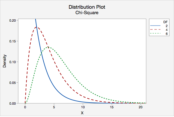
Like the t distribution, the chi-square distribution varies depending on the degrees of freedom. Degrees of freedom for a chi-square goodness-of-fit test are equal to the number of groups minus 1. The distribution plot below compares the chi-square distributions with 2, 4, and 6 degrees of freedom.
To find the p-value we find the area under the chi-square distribution to the right of our test statistic. A chi-square test is always right-tailed.
11.2.1 - Five Step Hypothesis Testing Procedure
11.2.1 - Five Step Hypothesis Testing ProcedureThe examples on the following pages use the five step hypothesis testing procedure outlined below. This is the same procedure that we used to conduct a hypothesis test for a single mean, single proportion, difference in two means, and difference in two proportions.
When conducting a chi-square goodness-of-fit test, it makes the most sense to write the hypotheses first. The hypotheses will depend on the research question. The null hypothesis will always contain the equalities and the alternative hypothesis will be that at least one population proportion is not as specified in the null.
In order to use the chi-square distribution to approximate the sampling distribution, all expected counts must be at least five.
- Expected Count
- \(E=np_i\)
-
Where \(n\) is the total sample size and \(p_i\) is the hypothesized population proportion in the "ith" group.
To check this assumption, compute all expected counts and confirm that each is at least five.
In Step 1 you already computed the expected counts. Use this formula to compute the chi-square test statistic:
- Chi-Square Test Statistic
- \(\chi^2=\sum \dfrac{(O-E)^2}{E}\)
- Where \(O\) is the observed count for each cell and \(E\) is the expected count for each cell.
Construct a chi-square distribution with degrees of freedom equal to the number of groups minus one. The p-value is the area under that distribution to the right of the test statistic that was computed in Step 2. You can find this area by constructing a probability distribution plot in Minitab.
Unless otherwise stated, use the standard 0.05 alpha level.
\(p \leq \alpha\) reject the null hypothesis.
\(p > \alpha\) fail to reject the null hypothesis.
Go back to the original research question and address it directly. If you rejected the null hypothesis, then there is evidence that at least one of the population proportions is not as stated in the null hypothesis. If you failed to reject the null hypothesis, then there is not enough evidence that any of the population proportions are different from what is stated in the null hypothesis.
11.2.1.1 - Video: Cupcakes (Equal Proportions)
11.2.1.1 - Video: Cupcakes (Equal Proportions)11.2.1.2- Cards (Equal Proportions)
11.2.1.2- Cards (Equal Proportions)Example: Cards
Research question: When randomly selecting a card from a deck with replacement, are we equally likely to select a heart, diamond, spade, and club?
I randomly selected a card from a standard deck 40 times with replacement. I pulled 13 hearts, 8 diamonds, 8 spades, and 11 clubs.
Let's use the five-step hypothesis testing procedure:
\(H_0: p_h=p_d=p_s=p_c=0.25\)
\(H_a:\) at least one \(p_i\) is not as specified in the null
We can use the null hypothesis to check the assumption that all expected counts are at least 5.
\(Expected\;count=n (p_i)\)
All \(p_i\) are 0.25. \(40(0.25)=10\), thus this assumption is met and we can approximate the sampling distribution using the chi-square distribution.
\(\chi^2=\sum \dfrac{(Observed-Expected)^2}{Expected} \)
All expected values are 10. Our observed values were 13, 8, 8, and 11.
\(\chi^2=\dfrac{(13-10)^2}{10}+\dfrac{(8-10)^2}{10}+\dfrac{(8-10)^2}{10}+\dfrac{(11-10)^2}{10}\)
\(\chi^2=\dfrac{9}{10}+\dfrac{4}{10}+\dfrac{4}{10}+\dfrac{1}{10}\)
\(\chi^2=1.8\)
Our sampling distribution will be a chi-square distribution.
\(df=k-1=4-1=3\)
We can find the p-value by constructing a chi-square distribution with 3 degrees of freedom to find the area to the right of \(\chi^2=1.8\)
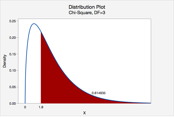
The p-value is 0.614935
\(p>0.05\) therefore we fail to reject the null hypothesis.
There is not enough evidence to state that the proportion of hearts, diamonds, spades, and clubs that are randomly drawn from this deck are different.
11.2.1.3 - Roulette Wheel (Different Proportions)
11.2.1.3 - Roulette Wheel (Different Proportions)Example: Roulette Wheel
Research Question: An American roulette wheel contains 38 slots: 18 red, 18 black, and 2 green. A casino has purchased a new wheel and they want to know if there is any evidence that the wheel is unfair. They spin the wheel 100 times and it lands on red 44 times, black 49 times, and green 7 times.
If the wheel is fair then \(p_{red}=\dfrac{18}{38}\), \(p_{black}=\dfrac{18}{38}\), and \(p_{green}=\dfrac{2}{38}\).
All of these proportions combined equal 1.
\(H_0: p_{red}=\dfrac{18}{38},\;p_{black}=\dfrac{18}{38}\;and\;p_{green}=\dfrac{2}{38}\)
\(H_a: At\;least\;one\;p_i\;is \;not\;as\;specified\;in\;the\;null\)
In order to conduct a chi-square goodness of fit test all expected values must be at least 5.
For both red and black: \(Expected \;count=100(\dfrac{18}{38})=47.368\)
For green: \(Expected\;count=100(\dfrac{2}{38})=5.263\)
All expected counts are at least 5 so we can conduct a chi-square goodness of fit test.
\(\chi^2=\sum \dfrac{(Observed-Expected)^2}{Expected} \)
In the first step we computed the expected values for red and black to be 47.368 and for green to be 5.263.
\(\chi^2= \dfrac{(44-47.368)^2}{47.368}+\dfrac{(49-47.368)^2}{47.368}+\dfrac{(7-5.263)^2}{5.263} \)
\(\chi^2=0.239+0.056+0.573=0.868\)
Our sampling distribution will be a chi-square distribution.
\(df=k-1=3-1=2\)
We can find the p-value by constructing a chi-square distribution with 2 degrees of freedom to find the area to the right of \(\chi^2=0.868\)
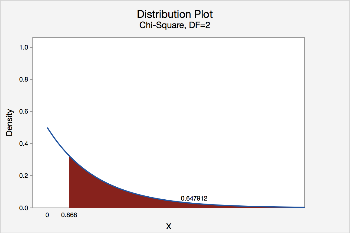
The p-value is 0.647912
\(p>0.05\) therefore we should fail to reject the null hypothesis.
There is not enough evidence that this roulette wheel is unfair.
11.2.2 - Minitab: Goodness-of-Fit Test
11.2.2 - Minitab: Goodness-of-Fit TestExample: Cards
Research Question: When randomly selecting a card from a deck with replacement, are we equally likely to select a heart, diamond, spade, and club?
I randomly selected a card from a standard deck 40 times with replacement. I pulled 13 Hearts (♥), 8 Diamonds (♦), 8 Spades (♠), and 11 Clubs (♣).
Minitab® – Conducting a Chi-Square Goodness-of-Fit Test
Summarized Data, Equal Proportions
To perform a chi-square goodness-of-fit test in Minitab using summarized data we first need to enter the data into the worksheet. Below you can see that we have one column with the names of each group and one column with the observed counts for each group.
| C1 | C2 | |
|---|---|---|
| Suit | Count | |
| 1 | Hearts | 13 |
| 2 | Diamonds | 8 |
| 3 | Spades | 8 |
| 4 | Clubs | 11 |
- After entering the data, select Stat > Tables > Chi-Square Goodness of Fit Test (One Variable)
- Double-click Count to enter it into the Observed Counts box
- Double-click Suit to enter it into the Category names (optional) box
- Click OK
This should result in the following output:
Chi-Square Goodness-of-Fit Test: Count
Observed and Expected Counts
| Category | Observed | Test Proportion |
Expected | Contribution to Chi-Sq |
|---|---|---|---|---|
| Hearts | 13 | 0.25 | 10 | 0.9 |
| Diamonds | 8 | 0.25 | 10 | 0.4 |
| Spades | 8 | 0.25 | 10 | 0.4 |
| Clubs | 11 | 0.25 | 10 | 0.1 |
Chi-Square Test
| N | DF | Chi-Sq | P-Value |
|---|---|---|---|
| 40 | 3 | 1.8 | 0.615 |
All expected values are at least 5 so we can use the chi-square distribution to approximate the sampling distribution. Our results are \(\chi^2 (3) = 1.8\). \(p = 0.615\). Because our p-value is greater than the standard alpha level of 0.05, we fail to reject the null hypothesis. There is not enough evidence to conclude that the proportions are different in the population.
Note!
The example above tested equal population proportions. Minitab also has the ability to conduct a chi-square goodness-of-fit test when the hypothesized population proportions are not all equal. To do this, you can choose to test specified proportions or to use proportions based on historical counts.
11.2.2.1 - Example: Summarized Data, Equal Proportions
11.2.2.1 - Example: Summarized Data, Equal ProportionsExample: Tulips
A company selling tulip bulbs claims they have equal proportions of white, pink, and purple bulbs and that they fill customer orders by randomly selecting bulbs from the population of all of their bulbs.
You ordered 30 bulbs and received 16 white, 8 pink, and 6 purple.
Is there evidence the bulbs you received were not randomly selected from a population with an equal proportion of each color?
Use Minitab to conduct a hypothesis test to address this research question.
We'll go through each of the steps in the hypotheses test:
\(H_0\colon p_{white}=p_{pink}=p_{purple}=\dfrac{1}{3}\)
\(H_a\colon\) at least one \(p_i\) is not \(\dfrac{1}{3}\)
We can use the null hypothesis to check the assumption that all expected counts are at least 5.
\(Expected\;count=n (p_i)\)
All \(p_i\) are \(\frac{1}{3}\). \(30(\frac{1}{3})=10\), thus this assumption is met and we can approximate the sampling distribution using the chi-square distribution.
Let's use Minitab to calculate this.
First, enter the summarized data into a Minitab Worksheet.
| C1 | C2 | |
|---|---|---|
| Color | Count | |
| 1 | White | 16 |
| 2 | Pink | 8 |
| 3 | Purple | 6 |
- After entering the data, select Stat > Tables > Chi-Square Goodness of Fit Test (One Variable)
- Double-click Count to enter it into the Observed Counts box
- Double-click Color to enter it into the Category names (optional) box
- Click OK
This should result in the following output:
Chi-Square Goodness-of-Fit Test: Count
Observed and Expected Counts
| Category | Observed | Test Proportion |
Expected | Contribution to Chi-Sq |
|---|---|---|---|---|
| White | 16 | 0.333333 | 10 | 3.6 |
| Pink | 8 | 0.333333 | 10 | 0.4 |
| Purple | 6 | 0.333333 | 10 | 1.6 |
Chi-Square Test
| N | DF | Chi-Sq | P-Value |
|---|---|---|---|
| 30 | 2 | 5.6 | 0.061 |
The test statistic is a Chi-Square of 5.6.
\(p>0.05\) therefore we fail to reject the null hypothesis.
There is not evidence that your tulip bulbs were not randomly selected from a population with equal proportions of white, pink and purple.
11.2.2.2 - Example: Summarized Data, Different Proportions
11.2.2.2 - Example: Summarized Data, Different ProportionsExample: Roulette
An American roulette wheel contains 38 slots: 18 red, 18 black, and 2 green. A casino has purchased a new wheel and they want to know if there is any evidence that the wheel is unfair. They spin the wheel 100 times and it lands on red 44 times, black 49 times, and green 7 times.
Use Minitab to conduct a hypothesis test to address this question.
We'll go through each of the steps in the hypotheses test:
If the wheel is 'fair' then the probability of red and black are both 18/38 and the probability of green is 2/38.
\(H_0\colon p_{red}=\dfrac{18}{38}, p_{black}=\dfrac{18}{38}, p_{green}=\dfrac{2}{38}\)
\(H_a\colon\) at least one \(p_i\) is not as specified in the null
We can use the null hypothesis to check the assumption that all expected counts are at least 5.
\(Expected\;count=n (p_i)\)
With n = 100 we meet the assumptions needed to use Chi-square.
Let's use Minitab to calculate this.
First, enter the summarized data into a Minitab Worksheet.
| C1 | C2 | |
|---|---|---|
| Color | Count | |
| 1 | Red | 44 |
| 2 | Black | 49 |
| 3 | Green | 7 |
- After entering the data, select Stat > Tables > Chi-Square Goodness of Fit Test (One Variable)
- Double-click Count to enter it into the Observed Counts box
- Double-click Color to enter it into the Category names (optional) box
- For Test select Input constants
- Select Proportions specified by historical counts (this is what we would expect if the null was true)
- Enter 18/38 for Black, 2/38 for Green and 18/38 for Red
- Click OK
This should result in the following output:
Chi-Square Goodness-of-Fit Test: Count
Observed and Expected Counts
| Category | Observed | Historical Counts | Test Proportion |
Expected | Contribution to Chi-Sq |
|---|---|---|---|---|---|
| Red | 44 | 18 | 0.473684 | 47.3684 | 0.239532 |
| Black | 49 | 18 | 0.473684 | 47.3684 | 0.056199 |
| Green | 7 | 2 | 0.052632 | 5.2632 | 0.573158 |
Chi-Square Test
| N | DF | Chi-Sq | P-Value |
|---|---|---|---|
| 100 | 2 | 0.868889 | 0.648 |
The test statistic is a Chi-Square of 0.87.
\(p>0.05\) therefore we fail to reject the null hypothesis.
There is not enough evidence to state that this roulette wheel is unfair.
11.3 - Chi-Square Test of Independence
11.3 - Chi-Square Test of IndependenceThe chi-square (\(\chi^2\)) test of independence is used to test for a relationship between two categorical variables. Recall that if two categorical variables are independent, then \(P(A) = P(A \mid B)\). The chi-square test of independence uses this fact to compute expected values for the cells in a two-way contingency table under the assumption that the two variables are independent (i.e., the null hypothesis is true).
Even if two variables are independent in the population, samples will vary due to random sampling variation. The chi-square test is used to determine if there is evidence that the two variables are not independent in the population using the same hypothesis testing logic that we used with one mean, one proportion, etc.
Again, we will be using the five step hypothesis testing procedure:
The assumptions are that the sample is randomly drawn from the population and that all expected values are at least 5 (we will see what expected values are later).
Our hypotheses are:
\(H_0:\) There is not a relationship between the two variables in the population (they are independent)
\(H_a:\) There is a relationship between the two variables in the population (they are dependent)
Note: When you're writing the hypotheses for a given scenario, use the names of the variables, not the generic "two variables."
- Chi-Square Test Statistic
- \(\chi^2=\sum \dfrac{(Observed-Expected)^2}{Expected}\)
- Expected Cell Value
- \(E=\dfrac{row\;total \; \times \; column\;total}{n}\)
The p-value can be found using Minitab. Look up the area to the right of your chi-square test statistic on a chi-square distribution with the correct degrees of freedom. Chi-square tests are always right-tailed tests.
- Degrees of Freedom: Chi-Square Test of Independence
- \(df=(number\;of\;rows-1)(number\;of\;columns-1)\)
If \(p \leq \alpha\) reject the null hypothesis.
If \(p>\alpha\) fail to reject the null hypothesis.
Write a conclusion in terms of the original research question.
11.3.1 - Example: Gender and Online Learning
11.3.1 - Example: Gender and Online LearningGender and Online Learning
A sample of 314 Penn State students was asked if they have ever taken an online course. Their genders were also recorded. The contingency table below was constructed. Use a chi-square test of independence to determine if there is a relationship between gender and whether or not someone has taken an online course.
| Have you taken an online course? | ||
|---|---|---|
| Yes | No | |
| Men | 43 | 63 |
| Women | 95 | 113 |
Solution
\(H_0:\) There is not a relationship between gender and whether or not someone has taken an online course (they are independent)
\(H_a:\) There is a relationship between gender and whether or not someone has taken an online course (they are dependent)
Looking ahead to our calculations of the expected values, we can see that all expected values are at least 5. This means that the sampling distribution can be approximated using the \(\chi^2\) distribution.
In order to compute the chi-square test statistic we must know the observed and expected values for each cell. We are given the observed values in the table above. We must compute the expected values. The table below includes the row and column totals.
| Have you taken an online course? | |||
|---|---|---|---|
| Yes | No | ||
| Men | 43 | 63 | 106 |
| Women | 95 | 113 | 208 |
| 138 | 176 | 314 | |
| \(E=\dfrac{row\;total \times column\;total}{n}\) |
| \(E_{Men,\;Yes}=\dfrac{106\times138}{314}=46.586\) |
| \(E_{Men,\;No}=\dfrac{106\times176}{314}=59.414\) |
| \(E_{Women,\;Yes}=\dfrac{208\times138}{314}=91.414\) |
| \(E_{Women,\;No}=\dfrac{208 \times 176}{314}=116.586\) |
Note that all expected values are at least 5, thus this assumption of the \(\chi^2\) test of independence has been met.
Observed and expected counts are often presented together in a contingency table. In the table below, expected values are presented in parentheses.
| Have you taken an online course? | |||
|---|---|---|---|
| Yes | No | ||
| Men | 43 (46.586) | 63 (59.414) | 106 |
| Women | 95 (91.414) | 113 (116.586) | 208 |
| 138 | 176 | 314 | |
\(\chi^2=\sum \dfrac{(O-E)^2}{E} \)
\(\chi^2=\dfrac{(43-46.586)^2}{46.586}+\dfrac{(63-59.414)^2}{59.414}+\dfrac{(95-91.414)^2}{91.414}+\dfrac{(113-116.586)^2}{116.586}=0.276+0.216+0.141+0.110=0.743\)
The chi-square test statistic is 0.743
\(df=(number\;of\;rows-1)(number\;of\;columns-1)=(2-1)(2-1)=1\)
We can determine the p-value by constructing a chi-square distribution plot with 1 degree of freedom and finding the area to the right of 0.743.
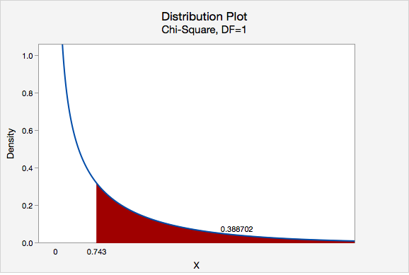
\(p = 0.388702\)
\(p>\alpha\), therefore we fail to reject the null hypothesis.
There is not enough evidence to conclude that gender and whether or not an individual has completed an online course are related.
Note that we cannot say for sure that these two categorical variables are independent, we can only say that we do not have enough evidence that they are dependent.
11.3.2 - Minitab: Test of Independence
11.3.2 - Minitab: Test of IndependenceRaw vs Summarized Data
If you have a data file with the responses for individual cases then you have "raw data" and can follow the directions below. If you have a table filled with data, then you have "summarized data." There is an example of conducting a chi-square test of independence using summarized data on a later page. After data entry the procedure is the same for both data entry methods.
Minitab® – Chi-square Test Using Raw Data
Research question: Is there a relationship between where a student sits in class and whether they have ever cheated?
- Null hypothesis: Seat location and cheating are not related in the population.
- Alternative hypothesis: Seat location and cheating are related in the population.
To perform a chi-square test of independence in Minitab using raw data:
- Open Minitab file: class_survey.mpx
- Select Stat > Tables > Chi-Square Test for Association
- Select Raw data (categorical variables) from the dropdown.
- Choose the variable Seating to insert it into the Rows box
- Choose the variable Ever_Cheat to insert it into the Columns box
- Click the Statistics button and check the boxes Chi-square test for association and Expected cell counts
- Click OK and OK
This should result in the following output:
Rows: Seating Columns: Ever_Cheat
| No | Yes | All | |
|---|---|---|---|
| Back | 24 | 8 | 32 |
| 24.21 | 7.79 | ||
| Front | 38 | 8 | 46 |
| 34.81 | 11.19 | ||
| Middle | 109 | 39 | 148 |
| 111.98 | 36.02 | ||
| All | 1714 | 55 | 226 |
Chi-Square Test
| Chi-Square | DF | P-Value | |
|---|---|---|---|
| Pearson | 1.539 | 2 | 0.463 |
| Likelihood Ratio | 1.626 | 2 | 0.443 |
Interpret
All expected values are at least 5 so we can use the Pearson chi-square test statistic. Our results are \(\chi^2 (2) = 1.539\). \(p = 0.463\). Because our \(p\) value is greater than the standard alpha level of 0.05, we fail to reject the null hypothesis. There is not enough evidence of a relationship in the population between seat location and whether a student has cheated.
11.3.2.1 - Example: Raw Data
11.3.2.1 - Example: Raw DataExample: Dog & Cat Ownership
Is there a relationship between dog and cat ownership in the population of all World Campus STAT 200 students? Let's conduct an hypothesis test using the dataset: fall2016stdata.mpx
\(H_0:\) There is not a relationship between dog ownership and cat ownership in the population of all World Campus STAT 200 students
\(H_a:\) There is a relationship between dog ownership and cat ownership in the population of all World Campus STAT 200 students
Assumption: All expected counts are at least 5. The expected counts here are 176.02, 75.98, 189.98, and 82.02, so this assumption has been met.
Let's use Minitab to calculate the test statistic and p-value.
- After entering the data, select Stat > Tables > Cross Tabulation and Chi-Square
- Enter Dog in the Rows box
- Enter Cat in the Columns box
- Select the Chi-Square button and in the new window check the box for the Chi-square test and Expected cell counts
- Click OK and OK
Rows: Dog Columns: Cat
| No | Yes | All | |
|---|---|---|---|
| No | 183 | 69 | 252 |
| 176.02 | 75.98 | ||
| Yes | 183 | 89 | 272 |
| 189.98 | 82.02 | ||
| Missing | 1 | 0 | |
| All | 366 | 158 | 524 |
Chi-Square Test
| Chi-Square | DF | P-Value | |
|---|---|---|---|
| Pearson | 1.771 | 1 | 0.183 |
| Likelihood Ratio | 1.775 | 1 | 0.183 |
Since the assumption was met in step 1, we can use the Pearson chi-square test statistic.
\(Pearson\;\chi^2 = 1.771\)
\(p = 0.183\)
Our p value is greater than the standard 0.05 alpha level, so we fail to reject the null hypothesis.
There is not enough evidence of a relationship between dog ownership and cat ownership in the population of all World Campus STAT 200 students.
11.3.2.2 - Example: Summarized Data
11.3.2.2 - Example: Summarized DataExample: Coffee and Tea Preference
Is there a relationship between liking tea and liking coffee?
The following table shows data collected from a random sample of 100 adults. Each were asked if they liked coffee (yes or no) and if they liked tea (yes or no).
| Likes Coffee | |||
|---|---|---|---|
| Yes | No | ||
| Likes Tea | Yes | 30 | 25 |
| No | 10 | 35 | |
Let's use the 5 step hypothesis testing procedure to address this research question.
\(H_0:\) Liking coffee an liking tea are not related (i.e., independent) in the population
\(H_a:\) Liking coffee and liking tea are related (i.e., dependent) in the population
Assumption: All expected counts are at least 5.
Let's use Minitab to calculate the test statistic and p-value.
- Enter the table into a Minitab worksheet as shown below:
C1 C2 C3 Likes Tea Likes Coffee-Yes Likes Coffee-No 1 Yes 30 25 2 No 10 35 - Select Stat > Tables > Cross Tabulation and Chi-Square
- Select Summarized data in a two-way table from the dropdown
- Enter the columns Likes Coffee-Yes and Likes Coffee-No in the Columns containing the table box
- For the row labels enter Likes Tea (leave the column labels blank)
- Select the Chi-Square button and check the boxes for Chi-square test and Expected cell counts.
- Click OK and OK
Output
Rows: Likes Tea Columns: Worksheet columns
| No | Yes | All | |
|---|---|---|---|
| Yes | 30 | 25 | 55 |
| 22 | 33 | ||
| No | 10 | 35 | 45 |
| 18 | 27 | ||
| All | 40 | 60 | 100 |
Chi-Square Test
| Chi-Square | DF | P-Value | |
|---|---|---|---|
| Pearson | 10.774 | 1 | 0.001 |
| Likelihood Ratio | 11.138 | 1 | 0.001 |
Since the assumption was met in step 1, we can use the Pearson chi-square test statistic.
\(Pearson\;\chi^2 = 10.774\)
\(p = 0.001\)
Our p value is less than the standard 0.05 alpha level, so we reject the null hypothesis.
There is evidence of a relationship between between liking coffee and liking tea in the population.
11.3.3 - Relative Risk
11.3.3 - Relative RiskA chi-square test of independence will give you information concerning whether or not a relationship between two categorical variables in the population is likely. As was the case with the single sample and two sample hypothesis tests that you learned earlier this semester, with a large sample size statistical power is high and the probability of rejecting the null hypothesis is high, even if the relationship is relatively weak. In addition to examining statistical significance by looking at the p value, we can also examine practical significance by computing the relative risk.
In Lesson 2 you learned that risk is often used to describe the probability of an event occurring. Risk can also be used to compare the probabilities in two different groups. First, we'll review risk, then you'll be introduced to the concept of relative risk.
The risk of an outcome can be expressed as a fraction or as the percent of a group that experiences the outcome.
- Risk
- \(Risk=\dfrac{n\;with\;outcome}{total\;n}\)
Examples of Risk
Asthma
60 out of 1000 teens have asthma. The risk is \(\frac{60}{1000}=.06\). This means that 6% of all teens experience asthma.
Flu
45 out of 100 children get the flu each year. The risk is \(\frac{45}{100}=.45\) or 45%
- Relative Risk
- Relative risk compares the risk of a particular outcome in two different groups.
- Relative Risk
- \(Relative\ Risk=\dfrac{Risk\ in\ Group\ 1}{Risk\ in\ Group\ 2}\)
Thus, relative risk gives the risk for group 1 as a multiple of the risk for group 2.
Example of Relative Risk
Flu
Suppose that the risk of a child getting the flu this year is .45 and the risk of an adult getting the flu this year is .10. What is the relative risk of children compared to adults?
- \(Relative\;risk=\dfrac{.45}{.10}=4.5\)
Children are 4.5 times more likely than adults to get the flu this year.
Caution
Watch out for relative risk statistics where no baseline information is given about the actual risk. For instance, it doesn't mean much to say that beer drinkers have twice the risk of stomach cancer as non-drinkers unless we know the actual risks. The risk of stomach cancer might actually be very low, even for beer drinkers. For example, 2 in a million is twice the size of 1 in a million but is would still be a very low risk. This is known as the baseline with which other risks are compared.
11.4 - Lesson 11 Summary
11.4 - Lesson 11 SummaryObjectives
- Construct a chi-square probability distribution plot in StatKey or Minitab.
- Determine when a chi-square goodness-of-fit test and chi-square test of independence should be conducted.
- Compute and interpret expected counts.
- Conduct chi-square tests by hand and using Minitab.
- Calculate and interpret relative risk.
In this lesson you added two new statistical procedures to your repertoire: the chi-square goodness-of-fit test for one categorical variable and the chi-square test of independence for two variables. In the remaining weeks we will continue to learn more procedures.