12.6 - Correlation & Regression Example
12.6 - Correlation & Regression ExampleExample: Vertical jump to predict 40-yd dash time
Each spring in Indianapolis, IN the National Football League (NFL) holds its annual combine. The combine is a place for college football players to perform various athletic and psycholological tests in front of NFL scouts.
Two of the most recognized tests are the forty-yard dash and the vertical jump. The forty-yard dash is the most popular test of speed, while the vertical jump measures the lower body power of the athlete.
Football players train extensively to improve these tests. We want to determine if the two tests are correlated in some way. If an athlete is good at one will they be good at the other? In this particular example, we are going to determine if the vertical jump could be used to predict the forty-yard dash time in college football players at the NFL combine.
Data from the past few years were collected from a sample of 337 college football players who performed both the forty-yard dash and the vertical jump.
Solution
We can learn more about the relationship between these two variables using correlation and regression.
Is there an association?
The correlation is given in the Minitab output:
P-Value = <0.0001
The variables have a strong, negative association.
Can we predict 40-yd dash time from vertical jump height?
Next, we'll conduct the simple linear regression procedure to determine if our explanatory variable (vertical jump height) can be used to predict the response variable (40 yd time).
Assumptions
First, we'll check our assumptions to use simple linear regression.
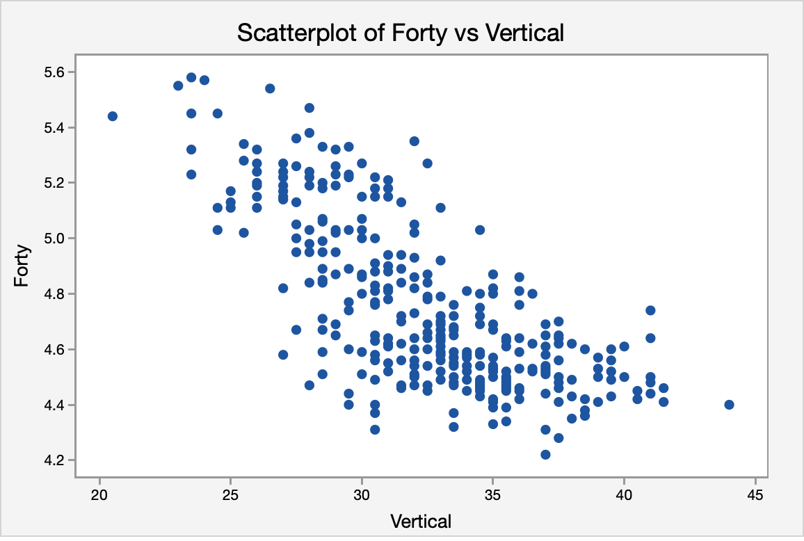
The scatterplot below shows a linear, moderately negative relationship between the vertical jump (in inches) and the forty-yard dash time (in seconds).
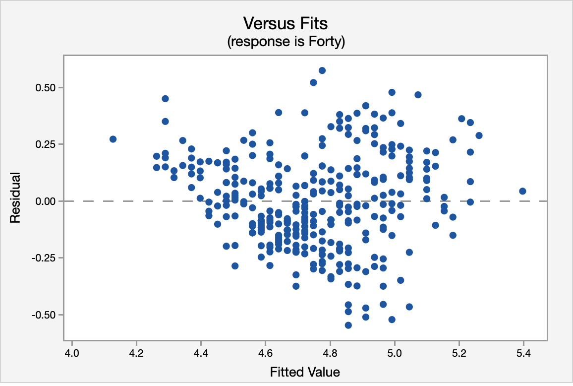
The correlation shown in the Versus Fits scatterplot is approximately 0. This assumption is met.

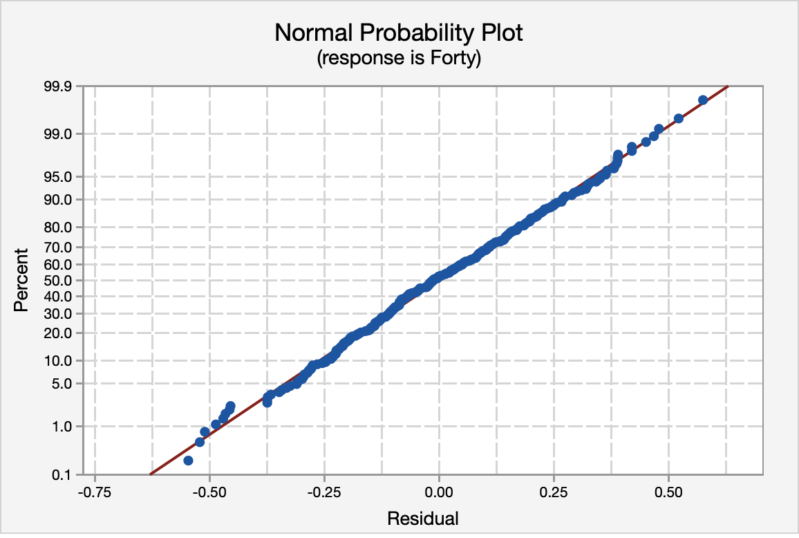
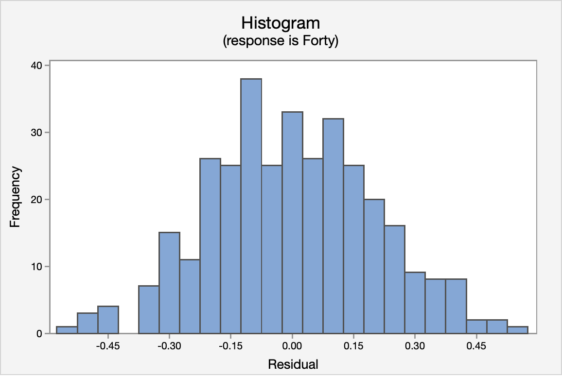
The normal probability plot and the histogram of the residuals confirm that the distribution of residuals is approximately normal.
Again, using the Versus Fits scatterplot we see no pattern among the residuals. We can assume equal variances.
ANOVA Table
The ANOVA source table gives us information about the entire model. The \(p\) value for the model is <0.0001. Because this is simple linear regression (SLR), this is the same \(p\) value that we found earlier when we examined the correlation and the same \(p\) value that we see below in the test of the statistical significance for the slope. Our \(R^2\) value is 0.5323 which tells us that 53.23% of the variance in forty-yard dash times can be explained by the vertical jump height of the athlete. This is a fairly good \(R^2\) for SLR.
Analysis of Variance
| Source | DF | Adj SS | Adj MS | F-Value | P-Value |
|---|---|---|---|---|---|
| Regression | 1 | 15.8872 | 15.8872 | 381.27 | <0.0001 |
| Error | 335 | 13.9591 | 0.0417 | ||
| Total | 336 | 29.8464 |
Model Summary
| S | R-sq | R-sq(adj) |
|---|---|---|
| 0.204130 | 53.23% | 53.09% |
Coefficients
| Predictor | Coef | SE Coef | T-Value | P-Value |
|---|---|---|---|---|
| Constant | 6.50316 | 0.09049 | 71.87 | <0.0001 |
| Vertical | -0.053996 | 0.002765 | -19.53 | <0.0001 |
Regression Equation
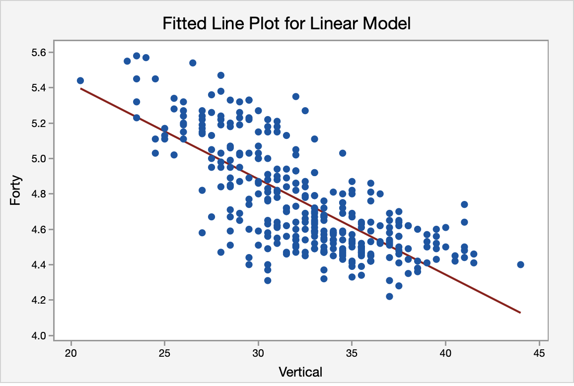
The regression equation for the two variables is:Forty = 6.50316 - 0.053996 Vertical
The regression equation indicates that for every inch gain in vertical jump height the 40-yd dash time will decrease by 0.053996 (the slope of the regression line). Finally, the fitted line plot shows us the regression equation on the scatter plot.