2.2 - One Quantitative Variable
2.2 - One Quantitative VariableOne quantitative variable is covered in Sections 2.2 and 2.3 of the Lock5 textbook. In these sections, you will learn how to describe the distribution of a quantitative variable in terms of shape, central tendency, and variability. You will be introduced to the normal distribution, z scores, percentiles, graphs, and the five-number-summary.
2.2.1 - Graphs: Dotplots and Histograms
2.2.1 - Graphs: Dotplots and HistogramsDotplots and histograms are both graphical displays that can be used with one quantitative variable. Below are descriptions for each along with some examples and instructions for constructing each in Minitab.
Dotplots
A dotplot can also be used to display data concerning one interval- or ratio-level variable. Each dot represents one, or more, data points. In the first example below, each dot represents one observation.
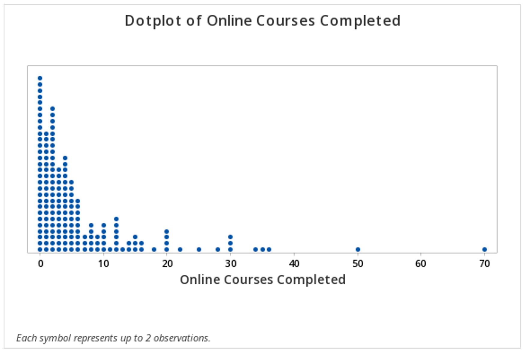
In this second example, the key at the bottom tells us that each dot may represent up to 2 observations.
Later in the course, in Lessons 4 and 5, we will study statistical inference and the application we will use will rely heavily on dotplots. For example, we will use dotplots to determine the proportion of points greater than, less than, or between two values. This can be determined by counting the dots.
Minitab® – Dotplot
This example will use data collected from a sample of students enrolled in online sections of STAT 200 during the Summer 2020 semester. These data can be downloaded as a CSV file:
To create a dotplot of the number of online courses completed:
- Open the data set in Minitab
- From the tool bar, select Graph > Dotplot...
- Under One Y Variable, select Simple
- Click OK
- Double click the variable Online Courses Completed in the box on the left to insert it into the Y-variable box on the right
- Click OK
This should result in the following dotplot:
Minitab®
Histograms
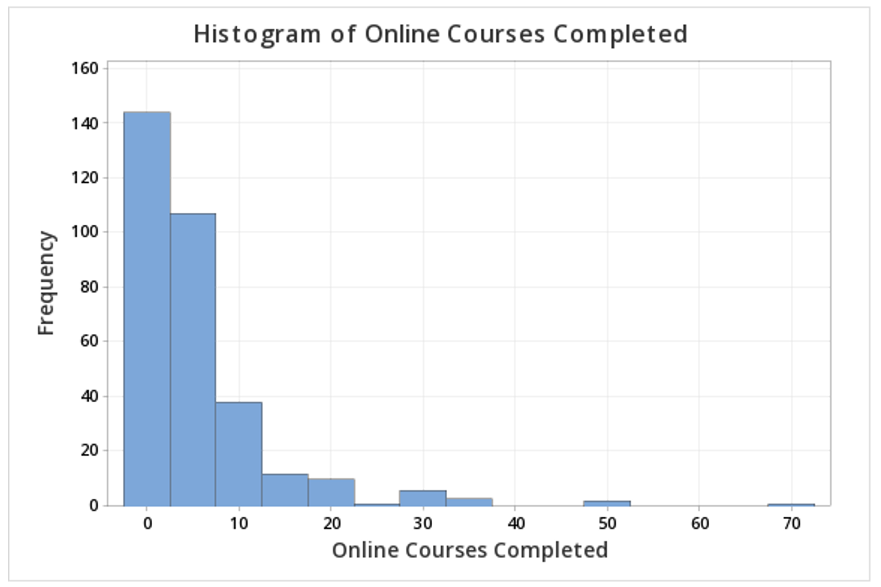
This example will use data collected from a sample of students enrolled in online sections of STAT 200 during the Summer 2020 semester. These data can be downloaded as a CSV file:
To create a histogram of the number of online courses completed in Minitab:
- Open the data set in Minitab
- From the tool bar, select Graph > Histogram...
- Under One Y Variable, select Simple
- Click OK
- Double click the variable Online Courses Completed in the box on the left to insert it into the Y-variable box on the right
- Click OK
This should result in the following histogram:
2.2.2 - Outliers
2.2.2 - OutliersSome observations within a set of data may fall outside the general scope of the other observations. Such observations are called outliers. Outliers can be identified by looking at a dotplot or histogram. In Lesson 3 you'll learn about boxplots which can also be used to identify outliers. When constructing a boxplot, Minitab identifies outliers using mathematical methods that you will see next week. This week we will identify outliers by making a relatively subjective judgement from a given a list of data points, a dotplot, or a histogram.
Example: Dotplot of Hours Watching TV
A sample of STAT 200 students was surveyed and asked how many hours per week they watch television. A dotplot was constructed using these data.
The right-most dot is definitely an outlier because it is much higher than any other points. The other higher points, around 55, 50, and 46, may be outliers. Next week we will learn about some mathematical methods for identifying outliers that can help us make decisions in cases like this where it is not obvious which values are outliers.
Example: Histogram of Best Marriage Age
This sample of students was also asked what they believed was the best age to get married. A histogram was constructed using these data.
There appear to be three outliers in this sample, all on the higher end.
2.2.3 - Shape
2.2.3 - ShapeQuantitative variables are often discussed in terms of their shape. Both dotplots and histograms can be used to interpret a distribution's shape. A distribution may be described in terms of symmetry and skewness.
- Symmetrical Distribution
-
A distribution that is similar on both sides of the center.
- Normal Distribution
-
One specific type of symmetrical distribution. This is also known as a bell-shaped distribution.
- Skewed
- A distribution in which values are more spread out on one side of the center than on the other.
- Right Skewed
-
A distribution in which the higher values (towards the right on a number line) are more spread out than the lower values. This is also known as positively skewed.
- Left Skewed
-
A distribution in which the lower values (towards the left on a number line) are more spread out than the higher values. This is also known as negatively skewed.
2.2.4 - Measures of Central Tendency
2.2.4 - Measures of Central TendencyQuantitative variables are often summarized using numbers to communicate their central tendency. The mean, median, and mode are three of the most commonly used measures of central tendency.
- Mean
-
The numerical average; calculated as the sum of all of the data values divided by the number of values.
The sample mean is represented as \(\overline{x}\) ("x-bar") and the population mean is denoted as the Greek letter \(\mu\) ("mu"). The formula is the same for the sample mean and the population mean.
- Population Mean
- \(\mu=\dfrac{\Sigma x}{N}\)
- Sample Mean
- \(\overline {x} = \dfrac{\Sigma x}{n}\)
- Median
- The middle of the distribution that has been ordered from smallest to largest; for distributions with an even number of values, this is the mean of the two middle values.
- Mode
- The most frequently occurring value(s) in the distribution, may be used with quantitative or categorical variables.
Example: Hours Spent Studying

A professor asks a sample of 7 students how many hours they spent studying for the final. Their responses are: 5, 7, 8, 9, 9, 11, and 13.
Mean
\(\overline{x} = \dfrac{\sum x}{n} =\dfrac{5+7+8+9+9+11+13}{7} =\dfrac{62}{7} =8.857\)
The mean is 8.857 hours.
Median
The observations are already in order from smallest to largest. The middle observation is 9 hours. The median is 9 hours.
Mode
The most frequently occurring observation was 9 hours. The mode is 9 hours.
In this example, the mean, median, and mode are all similar. Recall from our discussion of shape, the mean, median, and mode are all equal when a distribution is symmetric. This distribution of hours spent studying is probably close to symmetrical.
Example: Test Scores
A teacher wants to examine students’ test scores. Their scores are: 74, 88, 78, 90, 94, 90, 84, 90, 98, and 80.
Mean
\(\overline{x}\: =\: \dfrac{\sum x}{n} = \dfrac{74+88+78+90+94+90+84+90+98+80}{10} = \dfrac{866}{10}=86.6\)
The mean score was 86.6.
Median
First, we need to put the scores in order from lowest to highest: 74, 78, 80, 84, 88, 90, 90, 90, 94, 98
Because there is an even number of scores, the median will be the mean of the middle two values. The middle two values are 88 and 90. \(\frac{88+90}{2}=89\)
The median is 89.
Mode
The most frequently occurring score was 90. There were 3 students who scored a 90; this is the mode. Because this distribution has one mode, it is unimodal.
In this example the mean is slightly lower than the median which is slightly lower than the mode. Recall from our discussion of shape that this occurs when a distribution is skewed to the left. This distribution is probably slightly skewed to the left.
Example: Household Size
A group of children are asked how many people live in their household. The following data is collected: 4, 3, 6, 2, 2, 4, 3.
Mean
\(\overline{x} = \dfrac{\sum x}{n}=\dfrac{4+3+6+2+2+4+3}{7}=\dfrac{24}{7}=3.429\)
The mean household size in this group of children is 3.429 people.
Median
First, we need to put all of the values in order from smallest to largest: 2, 2, 3, 3, 4, 4, 6
The value in the middle of this distribution is 3. The median is 3.
Mode
In this distribution, the most common values are 2, 3, and 4. Each of these values occurs twice. There are 3 modes: 2, 3, and 4. This distribution is multimodal.
2.2.4.1 - Skewness & Central Tendency
2.2.4.1 - Skewness & Central TendencyThe preferred measure of central tendency often depends on the shape of the distribution. Of the three measures of tendency, the mean is most heavily influenced by any outliers or skewness.
In a symmetrical distribution, the mean, median, and mode are all equal. In these cases, the mean is often the preferred measure of central tendency.
For distributions that have outliers or are skewed, the median is often the preferred measure of central tendency because the median is more resistant to outliers than the mean. Below you will see how the direction of skewness impacts the order of the mean, median, and mode. Note that the mean is pulled in the direction of the skewness (i.e., the direction of the tail).
2.2.5 - Measures of Spread
2.2.5 - Measures of SpreadThe standard deviation is the most commonly used measure of variability when working with interval- or ratio-level variables. In a sample, this is denoted as \(s\). In a population, we use the Greek letter \(\sigma\) ("sigma").
When computing the standard deviation by hand, it is necessary to first compute the variance. The variance is equal to the standard deviation squared. In a sample, this is denoted as \(s^2\). In a population, it is \(\sigma^2\).
On this page we will provide some examples of computing standard deviation and variance by hand, but after this lesson you will always compute the standard deviation and variance using software such as Minitab.
- Sample Standard Deviation
- \(s=\sqrt{\dfrac{\sum (x-\overline{x})^{2}}{n-1}}\)
There are a number of methods for calculating the standard deviation. If you look through different textbooks or search online, you may find different formulas and procedures. To compute the standard deviation for a sample, we will use the formulas above and the following steps:
Step 1: Compute the sample mean: \(\overline{x} = \dfrac{\sum x}{n}\).
Step 2: Subtract the sample mean from each individual value: \(x-\overline{x}\), these are the deviations.
Step 3: Square each deviation: \((x-\overline{x})^{2}\), these are the squared deviations.
Step 4: Add the squared deviations: \(\sum (x-\overline{x})^{2}\), this is the sum of squares.
Step 5: Divide the sum of squares by \(n-1\): \(\frac{\sum (x-\overline{x})^{2}}{n-1}\), this is the sample variance \((s^{2})\).
Step 6: Take the square root of the sample variance: \(\sqrt{\frac{\sum (x-\overline{x})^{2}}{n-1}}\), this is the sample standard deviation (\(s\)).
The formula for computing the standard deviation in a population is slightly different. Note that the denominator chances from \(n-1\) to \(N\). In this course, we will primarily be using the sample standard deviation, but you can review the following formulas to see the similarities.
- Population Standard Deviation
- \(\sigma=\sqrt{\dfrac{\sum (x-\mu)^{2}}{N}}\)
- Sample Variance
- \(s^2=\dfrac{\sum (x-\overline{x})^{2}}{n-1}\)
- Population Variance
- \(\sigma^2=\dfrac{\sum (x-\mu)^{2}}{N}\)
Video Example
The video below walks through an example of computing a sample standard deviation by hand.
Example: Hours Spent Studying

A professor asks a sample of 7 students how many hours they spent studying for the final. Their responses are: 5, 7, 8, 9, 9, 11, and 13.
Step 1: Compute the mean
\(\overline{x} = \dfrac{\sum x}{n}=\dfrac{5+7+8+9+9+11+13}{7}=8.857\)
Step 2: Compute the deviations
| \(x\) | \(x - \overline{x}\) |
|---|---|
| 5 | \(5 - 8.857 = -3.857\) |
| 7 | \(7 - 8.857 = -1.857\) |
| 8 | \(8 - 8.857 = -0.857\) |
| 9 | \(9 - 8.857 = 0.143\) |
| 9 | \(9 - 8.857 = 0.143\) |
| 11 | \(11 - 8.857 = 2.143\) |
| 13 | \(13 - 8.857 = 4.143\) |
Step 3: Square the deviations
| \(x\) | \(x - \overline{x}\) | \((x-\overline{x})^{2}\) |
|---|---|---|
| 5 | \(5 - 8.857 = -3.857\) | \(-3.857^{2} = 14.876\) |
| 7 | \(7 - 8.857 = -1.857\) | \(-1.857^{2} = 3.448\) |
| 8 | \(8 - 8.857 = -0.857\) | \(-0.857^{2} = 0.734\) |
| 9 | \(9 - 8.857 = 0.143\) | \(0.143^{2} = 0.0020\) |
| 9 | \(9 - 8.857 = 0.143\) | \(0.143^{2} = 0.0020\) |
| 11 | \(11 - 8.857 = 2.143\) | \(2.143^{2} = 4.592\) |
| 13 | \(13 - 8.857 = 4.143\) | \(4.143^{2} = 17.164\) |
Step 4: Sum the squared deviations
\(SS=\sum (x-\overline{x})^{2}=14.876+3.448+0.734+.020+.020+4.592+17.164=40.854\)
The sum of squares is 40.854
Step 5: Divide by n - 1 to compute the variance
\(s^{2}=\dfrac{\sum (x-\overline{x})^{2}}{n-1}=\dfrac{40.854}{7-1}=6.809\)
The variance is 6.809
Step 6: Take the square root of the variance
\(s=\sqrt{s^{2}}=\sqrt{6.809}=2.609\)
The standard deviation is 2.609
2.2.6 - Minitab: Central Tendency & Variability
2.2.6 - Minitab: Central Tendency & VariabilityMinitab may be used to compute descriptive statistics for numeric variables, including the mean, median, mode, standard deviation, and variance.
Note that these are the default setting in Minitab:
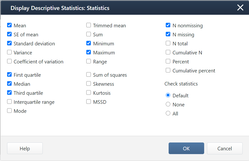
If you want additional statistics, such as the mode, variance, range, or interquartile range (IQR), you will need to select them in the Statistics window.
Minitab® – Central Tendency
Central Tendency and Variability
This example will use data collected from a sample of students enrolled in online sections of STAT 200 during the Summer 2020 semester. These data can be downloaded as a CSV file:
To obtain measures of central tendency and variability in Minitab:
- Open the data set in Minitab
- From the tool bar, select Stat > Basic Statistics > Display Descriptive Statistics...
- Double click the variable Online Courses Completed in the box on the left to insert it into the Variables box on the right
- Click on the Statistics button and select the descriptive statistics you want displayed (e.g., Variance, Interquartile range, Mode)
- Click OK
- Click OK
This should result in the following output:
| Variable | N | N* | Mean | SE Mean | StDev | Variance | Minimum | Q1 | Median | Q3 | Maximum | IQR | Mode | N for Mode |
|---|---|---|---|---|---|---|---|---|---|---|---|---|---|---|
| Online Courses Completed | 324 | 19 | 5.6975 | 0.4579 | 8.2429 | 67.945 | 0.0000 | 1.0000 | 3.0000 | 6.0000 | 70.0000 | 5.000 | 0 | 57 |
2.2.7 - The Empirical Rule
2.2.7 - The Empirical RuleA normal distribution is symmetrical and bell-shaped.
The Empirical Rule is a statement about normal distributions. Your textbook uses an abbreviated form of this, known as the 95% Rule, because 95% is the most commonly used interval. The 95% Rule states that approximately 95% of observations fall within two standard deviations of the mean on a normal distribution.
- Normal Distribution
- A specific type of symmetrical distribution, also known as a bell-shaped distribution
- Empirical Rule
-
On a normal distribution about 68% of data will be within one standard deviation of the mean, about 95% will be within two standard deviations of the mean, and about 99.7% will be within three standard deviations of the mean
The normal curve showing the empirical rule.
- 95% Rule
- On a normal distribution approximately 95% of data will fall within two standard deviations of the mean; this is an abbreviated form of the Empirical Rule
Example: Pulse Rates

Suppose the pulse rates of 200 college men are bell-shaped with a mean of 72 and standard deviation of 6.
- About 68% of the men have pulse rates in the interval \(72\pm1(6)=[66, 78]\).
- About 95% of the men have pulse rates in the interval \(72\pm2(6)=[60, 84]\).
- About 99.7% of the men have pulse rates in the interval \(72\pm 3(6)=[54, 90]\).
Example: IQ Scores
IQ scores are normally distributed with a mean of 100 and a standard deviation of 15.
- About 68% of individuals have IQ scores in the interval \(100\pm 1(15)=[85,115]\).
- About 95% of individuals have IQ scores in the interval \(100\pm 2(15)=[70,130]\).
- About 99.7% of individuals have IQ scores in the interval \(100\pm 3(15)=[55,145]\).
2.2.8 - z-scores
2.2.8 - z-scoresOften we want to describe an observation in relation to the distribution of all observations. We can do this using a z-score. By converting observations to z-scores, we can compare observations from different distributions.
- z-score
-
Distance between an individual score and the mean in standard deviation units; also known as a standardized score.
- z-score
- \(z=\dfrac{x - \overline{x}}{s}\)
-
\(x\) = original data value
\(\overline{x}\) = mean of the original distribution
\(s\) = standard deviation of the original distribution
This equation could also be rewritten in terms of population values: \(z=\frac{x-\mu}{\sigma}\)
Later in the course, we will learn more about the z-distribution, which is a special case of the normal distribution.
- z-distribution
-
A bell-shaped distribution with a mean of 0 and standard deviation of 1, also known as the standard normal distribution.
Example: Milk
A study of 66,831 dairy cows found that the mean milk yield was 12.5 kg per milking with a standard deviation of 4.3 kg per milking (data from Berry, et al., 2013).
A cow produces 18.1 kg per milking. What is this cow’s z-score?
\(z=\frac{x-\overline{x}}{s} =\frac{18.1-12.5}{4.3}=1.302\)
This cow’s z-score is 1.302; her milk production was 1.302 standard deviations above the mean.
A cow produces 12.5 kg per milking. What is this cow’s z-score?
\(z=\frac{x-\overline{x}}{s} =\frac{12.5-12.5}{4.3}=0\)
This cow’s z-score is 0; her milk production was the same as the mean.
A cow produces 8 kg per milking. What is this cow’s z-score?
\(z=\frac{x-\overline{x}}{s} =\frac{8-12.5}{4.3}=-1.047\)
This cow’s z-score is -1.047; her milk production was 1.047 standard deviations below the mean.
Berry, D. P., Coyne, J., Boughlan, B., Burke, M., McCarthy, J., Enright, B., Cromie, A. R., McParland, S. (2013). Genetics of milking characteristics in dairy cows. Animal, 7(11), 1750-1758.
Example: Comparing Test Scores
SAT-Math scores are normally distributed with a mean of 500 and standard deviation of 100. ACT-Math scores are normally distributed with a mean of 18 and standard deviation of 6. A student has taken both tests. They scored 600 on the SAT-Math and 22 on the ACT-Math. Which score is more impressive?
We can't directly compare the student's SAT and ACT scores because they are on different scales. We can convert these test scores into z-scores so we can directly compare them.
\(z_{SAT}=\frac{600-500}{100}=1\)
This student scored 1 standard deviation above the mean on the SAT-Math.
\(z_{ACT}=\frac{22-18}{6}=0.667\)
This student scored 0.667 standard deviations above the mean on the ACT-Math.
The student's SAT-Math score is more impressive than their ACT-Math score because the z-score is higher. They scored better than a larger proportion of other test takers on the SAT-Math.
2.2.9 - Percentiles
2.2.9 - PercentilesThere are slightly different definitions of percentiles and different statistical software and textbooks may use different formulas. In this course, we will be using the definition from your textbook:
- Percentile
- Proportion of a distribution less than a given value.
Example: Final Exam Scores
The dotplot below displays the final exam scores from a sample of 100 students. Estimate the 90th percentile.
Given that there are 100 dots on this plot, the 90th percentile will fall around the 90th and 91st points. We can estimate the 90th percentile by counting down 10 from the top. The point that is 10th from the top is 59. Thus, the 90th percentile in this sample is a score of 59 points.
2.2.10 - Five Number Summary
2.2.10 - Five Number SummaryA five number summary can be used to communicate some key descriptive statistics. It is comprised of five values, presented in the following order:
- Minimum: Smallest value
- First quartile (Q1): 25th percentile (value that separates the bottom 25% of the distribution from the top 75%)
- Median: Middle value (50th percentile)
- Third quartile (Q3): 75th percentile (value that separates the bottom 75% of the distribution from the top 25%)
- Maximum: Largest value
- Five Number Summary
- Minimum, Q1, Median, Q3, Maximum
Five number summaries are used to describe some of the key features of a distribution. Using the values in a five number summary we can also compute the range and interquartile range.
- Range
- The difference between the maximum and minimum values.
- Range
- \(Range = Maximum - Minimum\)
- Note:
- The range is heavily influenced by outliers. For this reason, the interquartile range is often preferred because it is resistant to outliers.
- Interquartile range (IQR)
- The difference between the first and third quartiles.
- Interquartile Range
- \(IQR = Q_3 - Q_1\)
Example: Hours Spent Studying

A professor asks a sample of students how many hours they spent studying for the final. The five number summary for their responses is (5, 7, 9, 11, 13).
Range
The maximum is 13 and the minimum is 5.
\(Range = 13 - 5 = 8\)
Interquartile Range
The third quartile is 11 and the first quartile is 7.
\(IQR = Q_3 - Q_1 = 11 - 7 = 4\)
Example: Test Scores
A teacher wants to examine students’ test scores. The five number summary for their scores is (74, 80, 89, 90, 98).
Range
The highest score is 98. The lowest score is 74.
\(Range = 98 - 74 = 24\)
Interquartile Range
The third quartile is 90 and the first quartile is 80.
\(IQR = Q3 - Q1 = 90 - 80 = 10\)