12.3.2 - Assumptions

Assumptions of Simple Linear Regression

In order to use the methods above, there are four assumptions that must be met:

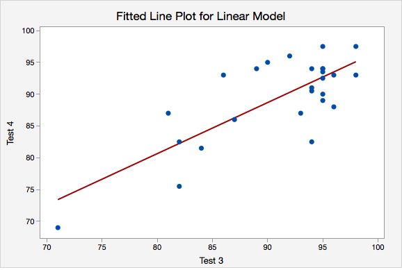
Linearity: The relationship between \(x\) and y must be linear. Check this assumption by examining a scatterplot of \(x\) and \(y\).
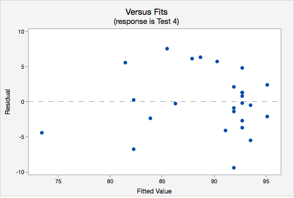
Independence of errors: There is not a relationship between the residuals and the predicted values. Check this assumption by examining a scatterplot of “residuals versus fits.” The correlation should be approximately 0.
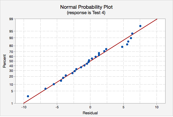
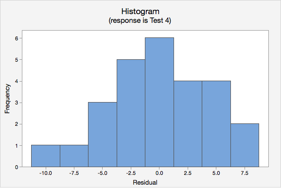
Normality of errors: The residuals must be approximately normally distributed. Check this assumption by examining a normal probability plot; the observations should be near the line. You can also examine a histogram of the residuals; it should be approximately normally distributed. The distribution will not be perfectly normal because we're working with sample data and there may be some sampling error, but the distribution should not be clearly skewed.
Equal variances: The variance of the residuals should be consistent across all predicted values. Check this assumption by examining the scatterplot of “residuals versus fits.” The variance of the residuals should be consistent across the x-axis. If the plot shows a pattern (e.g., bowtie or megaphone shape), then variances are not consistent and this assumption has not been met.

Example: Checking Assumptions

The following example uses students' scores on two tests.

Linearity. The scatterplot below shows that the relationship between Test 3 and Test 4 scores is linear.
Independence of errors. The plot of residuals versus fits is shown below. The correlation shown in this scatterplot is approximately \(r=0\), thus this assumption has been met.
Normality of errors. On the normal probability plot we are looking to see if our observations follow the given line. This tells us that the distribution of residuals is approximately normal. We could also look at the second graph which is a histogram of the residuals; here we see that the distribution of residuals is approximately normal.
Equal variance. Again we will use the plot of residuals versus fits. Now we are checking that the variance of the residuals is consistent across all fitted values.