Lesson 6: Bayes' Theorem
Lesson 6: Bayes' TheoremOverview
In this lesson, we'll learn about a classical theorem known as Bayes' Theorem. In short, we'll want to use Bayes' Theorem to find the conditional probability of an event \(P(A|B)\), say, when the "reverse" conditional probability \(P(B|A)\) is the probability that is known.
Objectives
- Learn how to find the probability of an event by using a partition of the sample space \(\mathbf{S}\).
- Learn how to apply Bayes' Theorem to find the conditional probability of an event when the "reverse" conditional probability is the probability that is known.
6.1 - An Example
6.1 - An ExampleExample 6-1
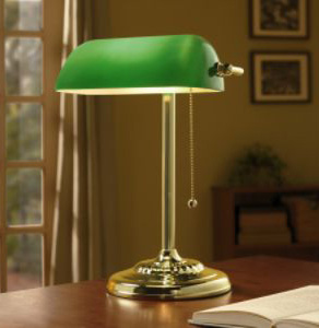
A desk lamp produced by The Luminar Company was found to be defective (\(D\)). There are three factories (\(A, B, C\)) where such desk lamps are manufactured. A Quality Control Manager (QCM) is responsible for investigating the source of found defects. This is what the QCM knows about the company's desk lamp production and the possible source of defects:
| Factory | % of total production | Probability of defective lamps |
| \(A\) | \(0.35=P(A)\) | \(0.015=P(D|A)\) |
| \(B\) | \(0.35=P(B)\) | \(0.010=P(D|B)\) |
| \(C\) | \(0.30=P(C)\) | \(0.020=P(D|C)\) |
The QCM would like to answer the following question: If a randomly selected lamp is defective, what is the probability that the lamp was manufactured in factory \(C\)?
Now, if a randomly selected lamp is defective, what is the probability that the lamp was manufactured in factory \(A\)? And, if a randomly selected lamp is defective, what is the probability that the lamp was manufactured in factory \(B\)?
Answer
In our previous work, we determined that \(P(D)\), the probability that a lamp manufactured by The Luminar Company is defective, is 0.01475. In order to find \(P(A|D)\) and \(P(B|D)\) as we are asked to find here, we need to perform a similar calculation to the one we used in finding \(P(C|D)\). Our work here will be simpler, though, since we've already done the hard work of finding \(P(D)\). The probability that a lamp was manufactured in factory A given that it is defective is:
\(P(A|D)=\dfrac{P(A\cap D)}{P(D)}=\dfrac{P(D|A)\times P(A)}{P(D)}=\dfrac{(0.015)(0.35)}{0.01475}=0.356\)
And, the probability that a lamp was manufactured in factory \(B\) given that it is defective is:
\(P(B|D)=\dfrac{P(B\cap D)}{P(D)}=\dfrac{P(D|B)\times P(B)}{P(D)}=\dfrac{(0.01)(0.35)}{0.01475}=0.237\)
Note that in each case we effectively turned what we knew upside down on its head to find out what we really wanted to know! We wanted to find \(P(A|D)\), but we knew \(P(D|A)\). We wanted to find \(P(B|D)\), but we knew \(P(D|B)\). We wanted to find \(P(C|D)\), but we knew \(P(D|C)\).It is for this reason that I like to say that we are interested in finding "reverse conditional probabilities" when we solve such problems.
The probabilities \(P(A), P(B),\text{ and }P(C)\) are often referred to as prior probabilities, because they are the probabilities of events \(A\), \(B\), and \(C\) that we know prior to obtaining any additional information. The conditional probabilities \(P(A|D)\), \(P(B|D)\), and \(P(C|D)\) are often referred to as posterior probabilities, because they are the probabilities of the events after we have obtained additional information.
As a result of our work, we determined:
- \(P(C | D) = 0.407\)
- \(P(B | D) = 0.237\)
- \(P(A | D) = 0.356\)
Calculated posterior probabilities should make intuitive sense, as they do here. For example, the probability that the randomly selected desk lamp was manufactured in Factory \(C\) has increased, that is, \(P(C|D)>P(C)\), because Factory \(C\) generates the greatest proportion of defective lamps (\(P(D|C)=0.02\)). And, the probability that the randomly selected desk lamp was manufactured in Factory \(B\) has decreased, that is, \(P(B|D)<P(B)\), because Factory \(B\) generates the smallest proportion of defective lamps (\(P(D|B)=0.01\)). It is, of course, always a good practice to make sure that your calculated answers make sense.
Let's now go and generalize the kind of calculation we made here in this defective lamp example .... in doing so, we summarize what is called Bayes' Theorem.
6.2 - A Generalization
6.2 - A GeneralizationLet the \(m\) events \(B_1, B_2, \ldots, B_m\) constitute a partition of the sample space \(\mathbf{S}\). That is, the \(B_i\) are mutually exclusive:
\(B_i\cap B_j=\emptyset\) for \(i\ne j\)
and exhaustive:
\(\mathbf{S}=B_1\cup B_2\cup \ldots B_m\)
Also, suppose the prior probability of the event \(B_i\)is positive, that is, \(P(B_i)>0\) for \(i=1, \ldots, m\). Now, if \(A\) is an event, then \(A\) can be written as the union of \(m\) mutually exclusive events, namely:
\(A=(A\cap B_1)\cup(A\cap B_2)\cup\ldots\cup (A\cap B_m)\)
Therefore:
\begin{align} P(A) &= P(A\cap B_1)+P(A\cap B_2)+\ldots +P(A\cap B_m)\\ &= \sum\limits_{i=1}^m P(A\cap B_i)\\ &= \sum\limits_{i=1}^m P(B_i) \times P(A|B_i)\\ \end{align}
And so, as long as \(P(A)>0\), the posterior probability of event \(B_k\) given event \(A\) has occurred is:
\(P(B_k|A)=\dfrac{P(B_k \cap A)}{P(A)}=\dfrac{P(B_k)\times P(A|B_k)}{\sum\limits_{i=1}^m P(B_i)\times P(A|B_i)}\)
Now, even though I've presented the formal Bayes' Theorem to you, as I should have, the reality is that I still find "reverse conditional probabilities" using the brute force method I presented in the example on the last page. That is, I effectively re-create Bayes' Theorem every time I solve such a problem.
6.3 - Another Example
6.3 - Another ExampleExample 6-2
A common blood test indicates the presence of a disease 95% of the time when the disease is actually present in an individual. Joe's doctor draws some of Joe's blood, and performs the test on his drawn blood. The results indicate that the disease is present in Joe.
Here's the information that Joe's doctor knows about the disease and the diagnostic blood test:
- One-percent (that is, 1 in 100) people have the disease. That is, if \(D\) is the event that a randomly selected individual has the disease, then \(P(D)=0.01\).
- If \(H\) is the event that a randomly selected individual is disease-free, that is, healthy, then \(P(H)=1-P(D)=0.99\).
- The sensitivity of the test is 0.95. That is, if a person has the disease, then the probability that the diagnostic blood test comes back positive is 0.95. That is, \P(T+|D)=0.95\).
- The specificity of the test is 0.95. That is, if a person is free of the disease, then the probability that the diagnostic test comes back negative is 0.95. That is, \(P(T-|H)=0.95\).
- If a person is free of the disease, then the probability that the diagnostic test comes back positive is \(1-P(T-|H)=0.05\). That is, \(P(T+|H)=0.05\).
What is the positive predictive value of the test? That is, given that the blood test is positive for the disease, what is the probability that Joe actually has the disease?
The test is seemingly not all that accurate! Even though Joe tested positive for the disease, our calculation indicates that he has only a 16% chance of actually having the disease. Is the test bogus? Should the test be discarded? Not at all! This kind of result is quite typical of screening tests in which the disease is fairly unusual. It is informative after all to know that, to begin with, not many people have the disease. Knowing that Joe has tested positive increases his chances of actually having the disease (from 1% to 16%), but the fact still remains that not many people have the disease. Therefore, it should still be fairly unlikely that Joe has the disease.
One strategy doctors often employ with inexpensive, not-too-invasive screening tests, such as Joe's blood test, is to perform the test again if the first test comes back positive. In that case, the population of interest is not all people, but instead those people who got a positive result on a first test. If a second blood test on Joe comes back positive for the disease, what is the probability that Joe actually has the disease now?
Incidentally, there is an alternative way of finding "reverse conditional probabilities," such as finding \(PD|T+)\), when you know the the "forward conditional probability" \(P(T+|D)\). Let's take a look:
Some Miscellaneous Comments
- It is quite common, even for people in the seeming know, to confuse forward and reverse conditional probabilities. A 1978 article in the New England Journal of Medicine reports how a problem similar to the one above was presented to 60 doctors at four Harvard Medical School teaching hospitals. Only eleven doctors gave the correct answer, and almost half gave the answer 95%.
- A person can be easily misled if he or she doesn't pay close attention to the difference between probabilities and conditional probabilities. As an example, consider that some people buy sport utility vehicles (SUV's) so that they will be safer on the road. In one way, they are actually correct. If they are in a crash, they would be safer in an SUV. (What kind of probability is this? A conditional probability!) Conditioned on an accident, the probability that a driver or passenger will be safe is better when in an SUV. But you might not necessarily care about this conditional probability. You might instead care more about the probability that you are in an accident. The probability that you are in an accident is actually higher when in an SUV! (What kind of probability is this? Just a probability, not conditioned on anything.) The moral of the story is that, when you draw conclusions, you need to make sure that you are using the right kind of probability to support your claim.
- The Reverend Thomas Bayes (1702-1761), a Nonconformist clergyman who rejected most of the rituals of the Church of England, did not publish his own theorem. It was only published posthumously after a friend had found it among Bayes' papers after his death. The theorem has since had an enormous influence on scientific and statistical thinking.
6.4 - More Examples
6.4 - More ExamplesExample 6-3
Bowl A contains 2 red chips; bowl B contains two white chips, and bowl C contains 1 red chip and 1 white chip. A bowl is selected at random, and one chip is taken at random from that bowl. What is the probability of selecting a white chip?
Answer
Let \(A\) be the event that Bowl A is randomly selected; let \(B\) be the event that Bowl B is randomly selected; and let \(C\) be the event that Bowl C is randomly selected. Because there are three bowls that are equally likely to be selected, \(P(A)=P(B)=P(C)=\dfrac{1}{3}\). Let W be the event that a white chip is randomly selected. The probability of selecting a white chip from a bowl depends on the bowl from which the chip is selected:
- \(P(W|A)=0\)
- \(P(W|B)=1\)
- \(P(W|C)=\dfrac{1}{2}\)
Now, a white chip could be selected in one of three ways: (1) Bowl A could be selected, and then a white chip be selected from it; or (2) Bowl B could be selected, and then a white chip be selected from it; or (3) Bowl C could be selected, and then a white chip be selected from it. That is, the probability that a white chip is selected is:
\(P(W)=P[(W\cap A)\cup (W\cap B)\cup (W\cap C)]\)
Then, recognizing that the events \(W\cap A\), \(W\cap B\), and \(W\cap C\) are mutually exclusive, while simultaneously applying the Multiplication Rule, we have:
\(P(W)=P(W|A)P(A)+P(W|B)P(B)+P(W|C)P(C)\)
Now, we just need to substitute in the numbers that we know. That is:
\(P(W)=\left(0\times \dfrac{1}{3}\right)+\left(1\times \dfrac{1}{3}\right)+\left(\dfrac{1}{2}\times \dfrac{1}{3}\right)=0+\dfrac{1}{3}+\dfrac{1}{6}=\dfrac{1}{2}\)
We have determined that the probability that a white chip is selected is \(\dfrac{1}{2}\).
If the selected chip is white, what is the probability that the other chip in the bowl is red?
Answer
The only bowl that contains one white chip and one red chip is Bowl C. Therefore, we are interested in finding \(P(C|W)\). We will use the fact that \(P(W)=\frac{1}{2}\), as determined by our previous calculation. Here is how the calculation for this problem works:
\(P(C|W)=\dfrac{P(C\cap W)}{P(W)}=\dfrac{P(W|C)P(C)}{P(W)}=\dfrac{\dfrac{1}{2}\times \dfrac{1}{3}}{\dfrac{1}{2}}=\dfrac{1}{3}\)
The first equal sign comes, of course, from the definition of conditional probability. The second equal sign comes from the Multiplication Rule. And, the third equal sign comes from just substituting in the values that we know. We've determined that the probability that the other chip in the bowl is red given that the selected chip is white is \(\dfrac{1}{3}\).
Example 6-4

Each bag in a large box contains 25 tulip bulbs. Three-fourths of the bags are of Type A containing bulbs for 5 red and 20 yellow tulips; one-fourth of the bags are of Type B contain bulbs for 15 red and 10 yellow tulips. A bag is selected at random and one bulb is planted. What is the probability that the bulb will produce a red tulip?
Answer
If \(A\) denotes the event that a Type A bag is selected, then, because 75% of the bags are of Type A, \(P(A)=0.75\). If \(B\) denotes the event that a Type B bag is selected, then, because 25% of the bags are of Type B, \(P(B)=0.25\). Let \(R\) denote the event that the selected bulb produces a red tulip. Then:
What is the probability that the bulb will produce a yellow tulip?
Answer
Let Y denote the event that the selected bulb produces a yellow tulip. Then:
If the tulip is red, what is the probability that a bag having 15 red and 10 yellow tulips was selected?