Section 2: Discrete Distributions
Section 2: Discrete DistributionsIn the previous section, we learned some basic probability rules, as well as some counting techniques that can be useful in determining the probability of an event using the classical approach. In this section, we'll explore discrete random variables and discrete probability distributions. The basic idea is that when certain conditions are met, we can derive formulas for calculating the probability of an event. Then, instead of returning to the basic probability rules we learned in the previous section to calculate the probability of an event, we can use the new formulas we derived, providing the certain conditions are met.
Lesson 7: Discrete Random Variables
Lesson 7: Discrete Random VariablesOverview
In this lesson, we'll learn about general discrete random variables and general discrete probability distributions. Then, we'll investigate one particular probability distribution called the hypergeometric distribution.
Objectives
- To learn the formal definition of a discrete random variable.
- To learn the formal definition of a discrete probability mass function.
- To understand the conditions necessary for using the hypergeometric distribution.
- To be able to use the probability mass function of a hypergeometric random variable to find probabilities.
- To be able to apply the material learned in this lesson to new problems.
7.1 - Discrete Random Variables
7.1 - Discrete Random VariablesExample 7-1

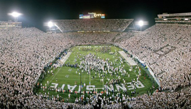
Select three fans randomly at a football game in which Penn State is playing Notre Dame. Identify whether the fan is a Penn State fan (\(P\)) or a Notre Dame fan (\(N\)). This experiment yields the following sample space:
\(\mathbf{S}=\{PPP, PPN, PNP, NPP, NNP, NPN, PNN, NNN\}\)
Let \(X\) = the number of Penn State fans selected. The possible values of \(X\) are, therefore, either 0, 1, 2, or 3. Now, we could find probabilities of individual events, \(P(PPP)\) or \(P(PPN)\), for example. Alternatively, we could find \(P(X=x)\), the probability that \(X\) takes on a particular value \(x\). Let's do that!
Since the game is a home game, let's suppose that 80% of the fans attending the game are Penn State fans, while 20% are Notre Dame fans. That is, \(P(P)=0.8\) and \(P(N)=0.2\). Then, by independence:
\(P(X=0)=P(NNN)=0.2\times0.2\times0.2=0.008\)
And, by independence and mutual exclusivity of \(NNP, NPN\), and \(PNN\):
\(P(X=1)=P(NNP)+P(NPN)+P(PNN)=3\times0.2\times0.2\times0.8=0.096\)
Likewise, by independence and mutual exclusivity of \(PPN, PNP\), and \(NPP\):
\(P(X=2)=P(PPN)+P(PNP)+P(NPP)=3\times0.8\times0.8\times0.2=0.384\)
Finally, by independence:
\(P(X = 3) = P(PPP) = 0.8\times0.8\times0.8 = 0.512\)
There are a few things to note here:
- The results make sense! Given that 80% of the fans in the stands are Penn State fans, it shouldn't seem surprising that we would be most likely to select 2 or 3 Penn State fans.
- The probabilities behave well in that (1) the probabilities are all greater than 0, that is, \(P(X=x)>0\) and (2) the probability of the sample space is 1, that is,\(P(\mathbf{S}) = P(X = 0) + P(X = 1) + P(X = 2) + P(X = 3) = 1\).
- Because the values that it takes on are random, the variable \(X\) has a special name. It is called a random variable! Ta-daaaa!
Let's give a formal definition of a random variable.
- Random Variable \(X\)
-
Given a random experiment with sample space \(\mathbf{S}\),a random variable \(X\) is a set function that assigns one and only one real number to each element \(s\) that belongs in the sample space \(\mathbf{S}\).
The set of all possible values of the random variable \(X\),denoted \(x\),is called the support, or space, of \(X\).
Note that the capital letters at the end of the alphabet, such as \(W, X, Y\), and \(Z\) typically represent the definition of the random variable. The corresponding lowercase letters, such as \(w, x, y\), and \(z\), represent the random variable's possible values.
Example 7-2
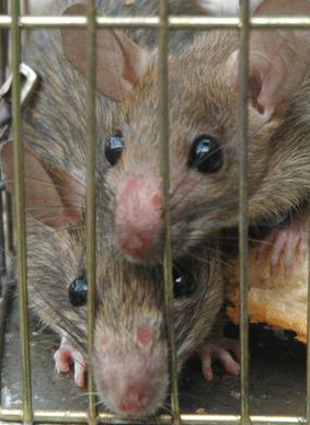
A rat is selected at random from a cage of male (\(M\)) and female rats (\(F\)). Once selected, the gender of the selected rat is noted. The sample space is thus:
\(\mathbf{S} = \{M, F\}\)
Define the random variable \(X\) as follows:
- Let \(X = 0\) if the rat is male.
- Let \(X = 1\) if the rat is female.
Note that the random variable \(X\) assigns one and only one real number (0 and 1) to each element of the sample space (\(M\) and \(F\)). The support, or space, of \(X\) is \(\{0, 1\}\).
Note that we don't necessarily need to use the numbers 0 and 1 as the support. For example, we could have alternatively (and perhaps arbitrarily?!) used the numbers 5 and 15, respectively. In that case, our random variable would be defined as \(X = 5\) of the rat is male, and \(X = 15\) if the rat is female.
Example 7-3
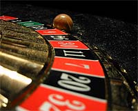
A roulette wheel has 38 numbers on it: a zero (0), a double zero (00), and the numbers 1, 2, 3, ..., 36. Spin the wheel until the pointer lands on number 36. One possibility is that the wheel lands on 36 on the first spin. Another possibility is that the wheel lands on 0 on the first spin, and 36 on the second spin. Yet another possibility is that the wheel lands on 0 on the first spin, 7 on the second spin, and 36 on the third spin. The sample space must list all of the countably infinite (!) number of possible sequences. That is, the sample space looks like this:
\(\mathbf{S} = \{36, 0-36, 00-36, 1-36, \ldots, 35-36, 0-0-36, 0-1-36, \ldots\}\)
If we define the random variable \(X\) to equal the number of spins until the wheel lands on 36, then the support of \(X\) is \(\{0, 1, 2, 3, \ldots\}\).
Note that in the rat example, there were a finite (two, to be exact) number of possible outcomes, while in the roulette example, there were a countably infinite number of possible outcomes. This leads us to the following formal definition.
- Discrete Random Variable
-
A random variable \(X\) is a discrete random variable if:
- there are a finite number of possible outcomes of \(X\), or
- there are a countably infinite number of possible outcomes of \(X\).
Recall that a countably infinite number of possible outcomes means that there is a one-to-one correspondence between the outcomes and the set of integers. No such one-to-one correspondence exists for an uncountably infinite number of possible outcomes.
As you might have guessed by its name, we will be studying discrete random variables and their probability distributions throughout Section 2.
7.2 - Probability Mass Functions
7.2 - Probability Mass FunctionsThe probability that a discrete random variable \(X\) takes on a particular value \(x\), that is, \(P(X = x)\), is frequently denoted \(f(x)\). The function \(f(x)\) is typically called the probability mass function, although some authors also refer to it as the probability function, the frequency function, or probability density function. We will use the common terminology — the probability mass function — and its common abbreviation —the p.m.f.
- Probability Mass Function
-
The probability mass function, \(P(X=x)=f(x)\), of a discrete random variable \(X\) is a function that satisfies the following properties:
- \(P(X=x)=f(x)>0\), if \(x\in \text{ the support }S\)
- \(\sum\limits_{x\in S} f(x)=1\)
- \(P(X\in A)=\sum\limits_{x\in A} f(x)\)
First item basically says that, for every element \(x\) in the support \(S\), all of the probabilities must be positive. Note that if \(x\) does not belong in the support \(S\), then \(f(x) = 0\). The second item basically says that if you add up the probabilities for all of the possible \(x\) values in the support \(S\), then the sum must equal 1. And, the third item says to determine the probability associated with the event \(A\), you just sum up the probabilities of the \(x\) values in \(A\).
Since \(f(x)\) is a function, it can be presented:
- in tabular form
- in graphical form
- as a formula
Let's take a look at a few examples.
Example 7-4
Let \(X\) equal the number of siblings of Penn State students. The support of \(X\) is, of course, 0, 1, 2, 3, ... Because the support contains a countably infinite number of possible values, \(X\) is a discrete random variable with a probability mass function. Find \(f(x) = P(X = x)\), the probability mass function of \(X\), for all \(x\) in the support.
This example illustrated the tabular and graphical forms of a p.m.f. Now let's take a look at an example of a p.m.f. in functional form.
Example 7-5
Let \(f(x)=cx^2\) for \(x = 1, 2, 3\). Determine the constant \(c\) so that the function \(f(x)\) satisfies the conditions of being a probability mass function.
Answer
The key to finding \(c\) is to use item #2 in the definition of a p.m.f.
The support in this example is finite. Let's take a look at an example in which the support is countably infinite.
Example 7-6
Determine the constant \(c\) so that the following p.m.f. of the random variable \(Y\) is a valid probability mass function:
\(f(y)=c\left(\dfrac{1}{4}\right)^y\) for y = 1, 2, 3, ...
Answer
Again, the key to finding \(c\) is to use item #2 in the definition of a p.m.f.
7.3 - The Cumulative Distribution Function (CDF)
7.3 - The Cumulative Distribution Function (CDF)The cumulative distribution function (CDF or cdf) of the random variable \(X\) has the following definition:
\(F_X(t)=P(X\le t)\)
The cdf is discussed in the text as well as in the notes but I wanted to point out a few things about this function. The cdf is not discussed in detail until section 2.4 but I feel that introducing it earlier is better. The notation sometimes confuses students. The notation \(F_X(t)\) means that \(F\) is the cdf for the random variable \(X\) but it is a function of \(t\).
We do not focus too much on the cdf for a discrete random variable but we will use them very often when we study continuous random variables. It does not mean that the cdf is not important for discrete random variables. They are just not always used since there are tables and software that help us to find these probabilities for common distributions.
The cdf of random variable \(X\) has the following properties:
- \(F_X(t)\) is a nondecreasing function of \(t\), for \(-\infty<t<\infty\).
- The cdf, \(F_X(t)\), ranges from 0 to 1. This makes sense since \(F_X(t)\) is a probability.
- If \(X\) is a discrete random variable whose minimum value is \(a\), then \(F_X(a)=P(X\le a)=P(X=a)=f_X(a)\). If \(c\) is less than \(a\), then \(F_X(c)=0\).
- If the maximum value of \(X\) is \(b\), then \(F_X(b)=1\).
- Also called the distribution function.
- All probabilities concerning \(X\) can be stated in terms of \(F\).
I have provided a few very brief examples using the cdf. We will be looking at these functions in more detail in the future.
Suppose \(X\) is a discrete random variable. Let the pmf of \(X\) be equal to
\(f(x)=\dfrac{5-x}{10}, \;\; x=1,2,3,4.\)
Suppose we want to find the cdf of \(X\). The cdf is \(F_X(t)=P(X\le t)\).
- For \(t=1\), \(P(X\le 1)=P(X=1)=f(1)=\dfrac{5-1}{10}=\dfrac{4}{10}\).
- For \(t=2\), \(P(X\le 2)=P(X=1 \text{ or } X=2)=P(X=1)+P(X=2)=\dfrac{5-1}{10}+\dfrac{5-2}{10}=\dfrac{4+3}{10}=\dfrac{7}{10}\)
- For \(t=3\), \(P(X\le 3)=\dfrac{5-1}{10}+\dfrac{5-2}{10}+\dfrac{5-3}{10}=\dfrac{4+3+1}{10}=\dfrac{9}{10}\).
- For \(t=4\), \(P(X\le 4)=\dfrac{5-1}{10}+\dfrac{5-2}{10}+\dfrac{5-3}{10}+\dfrac{5-4}{10}=\dfrac{10}{10}=1\).
It is worth noting that \(P(X\le 2)\) does not equal \(P(X<2)\); \(P(X\le 2)=P(X=1, 2)\) and \(P(X<2)=P(X=1)\). It is very important for you to carefully read the problems in order to correctly set up the probabilities. You should also look carefully at the notation if a problem provides it.
Consider \(X\) to be a random variable (a binomial random variable) with the following pmf
\(f(x)=P(X=x)={n\choose x}p^x(1-p)^{n-x}, \;\; \text{for } x=0, 1, \cdots , n.\)
The cdf of \(X\) evaluated at \(t\), denoted \(F_X(t)\), is
\(F_X(t)=\sum_{x=0}^t {n\choose x}p^x(1-p)^{n-x}, \;\; \text{for } 0\le t\le n.\)
- When \(t=0\), we have \(F_X(0)={n\choose 0}p^0(1-p)^{n-0}\).
- When \(t=1\), we have \(F_X(1)={n\choose 0}p^0(1-p)^{n-0}+{n\choose 1}p^1(1-p)^{n-1}\).
- When \(t=2\), we have \(F_X(2)={n\choose 0}p^0(1-p)^{n-0}+{n\choose 1}p^1(1-p)^{n-1}+ {n\choose 2}p^2(1-p)^{n-2}\).
And so on and so forth.
One last example. Suppose we have a family with three children. The sample space for this situation is
\(\mathbf{S}= \left \{ BBB, BBG, BGB, GBB, GGG, GGB, GBG, BGG \right \} \)
where \(B\) = boy and \(G\) = girl and suppose the probability of having a boy is the same as the probability of having a girl. Let the random variable \(X\) be the number of boys. Then \(X\) will have the following pmf:
| t | 0 | 1 | 2 | 3 |
| \(P(X=t)\) | \(\dfrac{1}{8}\) | \(\dfrac{3}{8}\) | \(\dfrac{3}{8}\) | \(\dfrac{1}{8}\) |
Then, we can use the pmf to find the cdf.
| t | 0 | 1 | 2 | 3 |
| \(F_X(t)=P(X\le t)\) | \(\dfrac{1}{8}\) | \(\dfrac{1}{8}+\dfrac{3}{8}=\dfrac{4}{8}\) | \(\dfrac{4}{8}+\dfrac{3}{8}=\dfrac{7}{8}\) | \(\dfrac{7}{8}+\dfrac{1}{8}=1\) |
Additional Practice Problem
These are some theoretical problems for the CDF and for expectations. Work these problems out on your own and then click on the link to view the solution.
- Express the following probabilities in terms of the cdf, \(F_X(t)\), if \(X\) is a discrete random variable with support such that \(x\) being any integer from 0 to \(b\) and \(0\le a\le b\):
-
\(P(X\le a)\)\(P(X\le a)=F_X(a)\) by definition of cdf
-
\(f_X(a)=P(X=a)\), where \(f_X(x)\) is the pmf of \(X\)\(P(X=a)=P(X\le a)-P(X\le a-1)=F_X(a)-F_X(a-1)\)
-
\(P(X<a)\)\(P(X<a)=P(X\le a)-P(X=a)=P(X\le a-1)=F_X(a-1)\)
-
\(P(X\ge a)\)\(P(X\ge a)=1-P(X\le a-1)=1-F_X(a-1)\)
-
-
Let \(X\) have distribution function \(F\). What is the distribution function and expectation of \(\dfrac{X - \mu}{\sigma}\)? In other words, find the distribution function in terms of \(F_X\) and the expectation in terms of \(E(X)\).
Let \(Y=\dfrac{X-\mu}{\sigma}\). We want \(F_Y(t)\) and \(E(Y)\).
\begin{align*} & F_Y(y)=P(Y\le y), \text{ by definition of cdf of Y}\\ & F_Y(y)=P(Y\le y)=P\left(\dfrac{X-\mu}{\sigma}\le y\right)=P\left(X\le y\sigma+\mu\right)\\ & F_Y(y)= F_X(t\sigma+\mu) \end{align*}
Now, to find the expectation, we can do this in two ways. One way is to find it using the definition of expectation, \(E(Y)=\sum_y yf_Y(y)\). In order to do this though, we would need to find \(f_Y(y)\), which we can find using the CDF if \(F_X\) was given.
The other way to approach this is to use the properties of expectation.
\(E(Y)=E\left(\dfrac{X-\mu}{\sigma}\right)=\dfrac{1}{\sigma}E(X-\mu)=\dfrac{E(X)-\mu}{\sigma}\)
7.4 - Hypergeometric Distribution
7.4 - Hypergeometric DistributionExample 7-7

A crate contains 50 light bulbs of which 5 are defective and 45 are not. A Quality Control Inspector randomly samples 4 bulbs without replacement. Let \(X\) = the number of defective bulbs selected. Find the probability mass function, \(f(x)\), of the discrete random variable \(X\).
This example is an example of a random variable \(X\) following what is called the hypergeometric distribution. Let's generalize our findings.
- Hypergeometric distribution
-
If we randomly select \(n\) items without replacement from a set of \(N\) items of which:
\(m\) of the items are of one type and \(N-m\) of the items are of a second typethen the probability mass function of the discrete random variable \(X\) is called the hypergeometric distribution and is of the form:
\(P(X=x)=f(x)=\dfrac{\dbinom{m}{x} \dbinom{N-m}{n-x}}{\dbinom{N}{n}}\)
where the support \(S\) is the collection of nonnegative integers x that satisfies the inequalities:
\(x\le n\) \(x\le m\) \(n-x\le N-m\)
Note that one of the key features of the hypergeometric distribution is that it is associated with sampling without replacement. We will see later, in Lesson 9, that when the samples are drawn with replacement, the discrete random variable \(X\) follows what is called the binomial distribution.
7.5 - More Examples
7.5 - More ExamplesExample 7-8

A lake contains 600 fish, eighty (80) of which have been tagged by scientists. A researcher randomly catches 15 fish from the lake. Find a formula for the probability mass function of \(X\), the number of fish in the researcher's sample which are tagged.
Solution
This problem is very similar to the example on the previous page in which we were interested in finding the p.m.f. of \(X\), the number of defective bulbs selected in a sample of 4 bulbs. Here, we are interested in finding \(X\), the number of tagged fish selected in a sample of 15 fish. That is, \(X\) is a hypergeometric random variable with \(m = 80\), \(N = 600\), and \(n = 15\). Therefore, the p.m.f. of \(X\) is:
for the support \(x=0, 1, 2, \ldots, 15\).
Example 7-9
Let the random variable \(X\) denote the number of aces in a five-card hand dealt from a standard 52-card deck. Find a formula for the probability mass function of \(X\).
Solution
The random variable \(X\) here also follows the hypergeometric distribution. Here, there are \(N=52\) total cards, \(n=5\) cards sampled, and \(m=4\) aces. Therefore, the p.m.f. of \(X\) is:
\(f(x)=\dfrac{\dbinom{4}{x} \dbinom{48}{5-x}}{\dbinom{52}{5}}\)
for the support \(x=0, 1, 2, 3, 4\).
Example 7-10

Suppose that 5 people, including you and a friend, line up at random. Let the random variable \(X\) denote the number of people standing between you and a friend. Determine the probability mass function of \(X\) in tabular form. Also, verify that the p.m.f. is a valid p.m.f.
Lesson 8: Mathematical Expectation
Lesson 8: Mathematical ExpectationOverview
In this lesson, we learn a general definition of mathematical expectation, as well as some specific mathematical expectations, such as the mean and variance.
Objectives
- To get a general understanding of the mathematical expectation of a discrete random variable.
- To learn a formal definition of \(E[u(X)]\), the expected value of a function of a discrete random variable.
- To understand that the expected value of a discrete random variable may not exist.
- To learn and be able to apply the properties of mathematical expectation.
- To learn a formal definition of the mean of a discrete random variable.
- To derive a formula for the mean of a hypergeometric random variable.
- To learn a formal definition of the variance and standard deviation of a discrete random variable.
- To learn and be able to apply a shortcut formula for the variance of a discrete random variable.
- To be able to calculate the mean and variance of a linear function of a discrete random variable.
- To learn a formal definition of the sample mean and sample variance.
- To learn and be able to apply a shortcut formula for the sample variance.
- To understand the steps involved in each of the proofs in the lesson.
- To be able to apply the methods learned in the lesson to new problems.
8.1 - A Definition
8.1 - A DefinitionExample 8-1

Toss a fair, six-sided die many times. In the long run (do you notice that it is bolded and italicized?!), what would the average (or "mean") of the tosses be? That is, if we have the following, for example:
| 1 | 3 | 2 | 4 | 5 | 6 | 5 | 4 | 4 | 1 | 2 | 3 |
|---|---|---|---|---|---|---|---|---|---|---|---|
| 2 | 1 | 3 | 6 | 4 | 5 | 5 | 4 | 3 | 1 | 6 | 6 |
| 2 | 5 | 3 | 1 | 2 | 4 | 6 | 2 | 5 | 6 | 3 | 1 |
what is the average of the tosses?
This example lends itself to a couple of notes.
- In reality, one-sixth of the tosses will equal \(x\) only in the long run (there's that bolding again).
- The mean is a weighted average, that is, an average of the values weighted by their respective individual probabilities.
- The mean is called the expected value of \(X\), denoted \(E(X)\) or by \(\mu\), the greek letter mu (read "mew").
Let's give a formal definition.
- Mathematical Expectation
-
If \(f(x)\) is the p.m.f. of the discrete random variable \(X\) with support \(S\), and if the summation:
\(\sum\limits_{x\in S}u(x)f(x)\)
exists (that is, it is less than \(\infty\)), then the resulting sum is called the mathematical expectation, or the expected value of the function \(u(X)\). The expectation is denoted \(E[u(X)]\). That is:
\(E[u(X)]=\sum\limits_{x\in S}u(x)f(x)\)
Example 8-2
What is the average toss of a fair six-sided die?
Solution
If the random variable \(X\) is the top face of a tossed, fair, six-sided die, then the p.m.f. of \(X\) is:
\(f(x)=\dfrac{1}{6}\)
for \(x=1, 2, 3, 4, 5, \text{and } 6\). Therefore, the average toss, that is, the expected value of \(X\), is:
\(E(X)=1\left(\dfrac{1}{6}\right)+2\left(\dfrac{1}{6}\right)+3\left(\dfrac{1}{6}\right)+4\left(\dfrac{1}{6}\right)+5\left(\dfrac{1}{6}\right)+6\left(\dfrac{1}{6}\right)=3.5\)
Hmm... if we toss a fair, six-sided die once, should we expect the toss to be 3.5? No, of course not! All the expected value tells us is what we would expect the average of a large number of tosses to be in the long run. If we toss a fair, six-sided die a thousand times, say, and calculate the average of the tosses, will the average of the 1000 tosses be exactly 3.5? No, probably not! But, we can certainly expect it to be close to 3.5. It is important to keep in mind that the expected value of \(X\) is a theoretical average, not an actual, realized one!
Example 8-3

Hannah's House of Gambling has a roulette wheel containing 38 numbers: zero (0), double zero (00), and the numbers 1, 2, 3, ..., 36. Let \(X\) denote the number on which the ball lands and \(u(X)\) denote the amount of money paid to the gambler, such that:
\begin{array}{lcl} u(X) &=& \$5 \text{ if } X=0\\ u(X) &=& \$10 \text{ if } X=00\\ u(X) &=& \$1 \text{ if } X \text{ is odd}\\ u(X) &=& \$2 \text{ if } X \text{ is even} \end{array}
How much would I have to charge each gambler to play in order to ensure that I made some money?
Solution
Assuming that the ball has an equally likely chance of landing on each number, the p.m.f of \(X\) is:
\(f(x)=\dfrac{1}{38}\)
for \(x=0, 00, 1, 2, 3, \ldots, 36\). Therefore, the expected value of \(u(X)\) is:
\(E(u(X))=\$5\left(\dfrac{1}{38}\right)+\$10\left(\dfrac{1}{38}\right)+\left[\$1\left(\dfrac{1}{38}\right)\times 18 \right]+\left[\$2\left(\dfrac{1}{38}\right)\times 18 \right]=\$1.82\)
Note that the 18 that is multiplied by the \$1 and \$2 is because there are 18 odd and 18 even numbers on the wheel. Our calculation tells us that, in the long run, Hannah's House of Gambling would expect to have to pay out \$1.82 for each spin of the roulette wheel. Therefore, in order to ensure that the House made money, the House would have to charge at least \$1.82 per play.
Example 8-4
Imagine a game in which, on any play, a player has a 20% chance of winning \$3 and an 80% chance of losing \$1. The probability mass function of the random variable \(X\), the amount won or lost on a single play is:
| x | \$3 | -\$1 |
| f(x) | 0.2 | 0.8 |
and so the average amount won (actually lost, since it is negative) — in the long run — is:
\(E(X)=(\$3)(0.2)+(-\$1)(0.8)=\$-0.20\)
What does "in the long run" mean? If you play, are you guaranteed to lose no more than 20 cents?
Solution
If you play and lose, you are guaranteed to lose \$1! An expected loss of 20 cents means that if you played the game over and over and over and over .... again, the average of your \$3 winnings and your \$1 losses would be a 20 cent loss. "In the long run" means that you can't draw conclusions about one or two plays, but rather thousands and thousands of plays.
Example 8-5
What is the expected value of a discrete random variable \(X\) with the following probability mass function:
\(f(x)=\dfrac{c}{x^2}\)
where \(c\) is a constant and the support is \(x=1, 2, 3, \ldots\)?
Solution
The expected value is calculated as follows:
\(E(X)=\sum\limits_{x=1}^\infty xf(x)=\sum\limits_{x=1}^\infty x\left(\dfrac{c}{x^2}\right)=c\sum\limits_{x=1}^\infty \dfrac{1}{x}\)
The first equal sign arises from the definition of the expected value. The second equal sign just involves replacing the generic p.m.f. notation \(f(x)\) with the given p.m.f. And, the third equal sign is because the constant \(c\) can be pulled through the summation sign, because it does not depend on the value of \(x\).
Now, to finalize our calculation, all we need to do is determine what the summation:
\(\sum\limits_{x=1}^\infty \dfrac{1}{x}\)
equals. Oops! You might recognize this quantity from your calculus studies as the divergent harmonic series, whose sum is infinity. Therefore, as the above definition of expectation suggests, we say in this case that the expected value of \(X\) doesn't exist.
This is the first example where the summation is not absolutely convergent. That is, we cannot get a finite answer here. The expectation for a random variable may not always exist. In this course, we will not encounter nonexistent expectations very often. However, when you encounter more sophisticated distributions in your future studies, you may find that the expectation does not exist.
8.2 - Properties of Expectation
8.2 - Properties of ExpectationExample 8-6
Suppose the p.m.f. of the discrete random variable \(X\) is:
| x | 0 | 1 | 2 | 3 |
| f(x) | 0.2 | 0.1 | 0.4 | 0.3 |
What is \(E(2)\)? What is \(E(X)\)? And, what is \(E(2X)\)?
This example leads us to a very helpful theorem.
- If \(c\) is a constant, then \(E(c)=c\)
- If \(c\) is a constant and \(u\) is a function, then:
\(E[cu(X)]=cE[u(X)]\)
Proof
Example 8-7
Let's return to the same discrete random variable \(X\). That is, suppose the p.m.f. of the random variable \(X\) is:
| x | 0 | 1 | 2 | 3 |
| f(x) | 0.2 | 0.1 | 0.4 | 0.3 |
It can be easily shown that \(E(X^2)=4.4\). What is \(E(2X+3X^2)\)?
This example again leads us to a very helpful theorem.
Let \(c_1\) and \(c_2\) be constants and \(u_1\) and \(u_2\) be functions. Then, when the mathematical expectation \(E\) exists, it satisfies the following property:
\(E[c_1 u_1(X)+c_2 u_2(X)]=c_1E[u_1(X)]+c_2E[u_2(X)]\)
Before we look at the proof, it should be noted that the above property can be extended to more than two terms. That is:
\(E\left[\sum\limits_{i=1}^k c_i u_i(X)\right]=\sum\limits_{i=1}^k c_i E[u_i(X)]\)
Proof
Example 8-8
Suppose the p.m.f. of the discrete random variable \(X\) is:
| x | 0 | 1 | 2 | 3 |
| f(x) | 0.2 | 0.1 | 0.4 | 0.3 |
In the previous examples, we determined that \(E(X)=1.8\) and \(E(X^2)=4.4\). Knowing that, what is \(E(4X^2)\) and \(E(3X+2X^2)\)?
Using part (b) of the first theorem, we can determine that:
\(E(4X^2)=4E(X^2)=4(4.4)=17.6\)
And using the second theorem, we can determine that:
\(E(3X+2X^2)=3E(X)+2E(X^2)=3(1.8)+2(4.4)=14.2\)
Example 8-9
Let \(u(X)=(X-c)^2\) where \(c\) is a constant. Suppose \(E[(X-c)^2]\) exists. Find the value of \(c\) that minimizes \(E[(X-c)^2]\).
Note that the expectations \(E(X)\) and \(E[(X-E(X))^2]\) are so important that they deserve special attention.
8.3 - Mean of X
8.3 - Mean of XIn the previous pages, we concerned ourselves with finding the expectation of any general function \(u(X)\) of the discrete random variable \(X\). Here, we'll focus our attention on one particular function, namely:
\(u(X)=X\)
Let's jump right in, and give the expectation in this situation a special name!
- First Moment about the Origin
-
When the function \(u(X)=X\), the expectation of \(u(X)\), when it exists:
\(E[u(X)]=E(X)=\sum\limits_{x\in S} xf(x) \)
is called the expected value of \(X\), and is denoted \(E(X)\). Or, it is called the mean of \(X\), and is denoted as \(\mu\) (the greek letter mu, read "mew"). That is, \(\mu=E(X)\). The expected value of \(X\) can also be called the first moment about the origin.
Example 8-10
The maximum patent life for a new drug is 17 years. Subtracting the length of time required by the Food and Drug Administration for testing and approval of the drug provides the actual patent life for the drug — that is, the length of time that the company has to recover research and development costs and to make a profit. The distribution of the lengths of actual patent lives for new drugs is as follows:
| Years, y | 3 | 4 | 5 | 6 | 7 | 8 | 9 | 10 | 11 | 12 | 13 |
|---|---|---|---|---|---|---|---|---|---|---|---|
| f(y) | 0.03 | 0.05 | 0.07 | 0.10 | 0.14 | 0.20 | 0.18 | 0.12 | 0.07 | 0.03 | 0.01 |
What is the mean patent life for a new drug?
Answer The mean can be calculated as:
\(\mu_Y=E(Y)=\sum\limits_{y=3}^{13} yf(y)=3(0.03)+4(0.05)+\cdots+12(0.03)+13(0.01)=7.9\)
That is, the average patent life for a new drug is 7.9 years.
Example 8-11
Let \(X\) follow a hypergeometric distribution in which n objects are selected from \(N\) objects with \(m\) of the objects being one type, and \(N-m\) of the objects being a second type. What is the mean of \(X\)?
Solution
Recalling the p.m.f. of a hypergeometric distribution and using the definition of the expected value of \(X\), we have:
\(E(X)=\sum\limits_{x\in S} x \dfrac{\dbinom{m}{x} \dbinom{N-m}{n-x}}{\dbinom{N}{n}}\)
You should be getting the idea already that this is going to be messy! So, we're going to work on it in parts. First, note that the first term of the summation equals 0 when \(x=0\). And, note that some of the terms can be written differently:
That is:
\(\dbinom{m}{x}=\dfrac{m!}{x!(m-x)!}\)
and:
\(\dbinom{N}{n}=\dfrac{N!}{n!(N-n)!}=\dfrac{N(N-1)!}{n \cdot (n-1)!(N-n)!}=\dfrac{N}{n} \cdot \dfrac{(N-1)!}{(n-1)!(N-1-(n-1))!}=\dfrac{N}{n} \cdot \dbinom{N-1}{n-1}\)
Therefore, replacing these quantities in our formula for \(E(X)\), we have:
My voice gets caught off at the end there, but we still managed to finish the proof in the nick of time! We've shown that, in general, the mean of a hypergeometric random variable \(X\), in which \(n\) objects are selected from \(N\) objects with \(m\) of the objects being one type, is:
\(E(X)=\dfrac{mn}{N}\)
Example 8-12
Suppose the random variable \(X\) follows the uniform distribution on the first \(m\) positive integers. That is, suppose the p.m.f. of \(X\) is:
\(f(x)=\dfrac{1}{m}\) for \(x=1, 2, 3, \ldots, m\)
What is the mean of \(X\)?
8.4 - Variance of X
8.4 - Variance of XExample 8-13
Consider two probability mass functions. The first:
| x | 3 | 4 | 5 |
|---|---|---|---|
| f(x) | 0.3 | 0.4 | 0.3 |
And, the second:
| y | 1 | 2 | 6 | 8 |
|---|---|---|---|---|
| f(y) | 0.4 | 0.1 | 0.3 | 0.2 |
It is a straightforward calculation to show that the mean of \(X\) and the mean of \(Y\) are the same:
\(\mu_X=E(X) = 3(0.3)+4(0.4)+5(0.3)=4\)
\(\mu_Y=E(Y)=1(0.4)+2(0.1)+6(0.3)+8(0.2)=4\)
Let's draw a picture that illustrates the two p.m.f.s and their means.
Again, the pictures illustrate (at least) two things:
- The \(X\) and \(Y\) means are at the fulcrums in which their axes don't tilt ("a balanced seesaw").
- The second p.m.f. exhibits greater variability than the first p.m.f.
That second point suggests that the means of \(X\) and \(Y\) are not sufficient in summarizing their probability distributions. Hence, the following definition!
Definition. When \(u(X)=(X-\mu)^2\), the expectation of \(u(X)\):
\(E[u(X)]=E[(X-\mu)^2]=\sum\limits_{x\in S} (x-\mu)^2 f(x)\)
is called the variance of \(X\), and is denoted as \(\text{Var}(X)\) or \(\sigma^2\) ("sigma-squared"). The variance of \(X\) can also be called the second moment of \(X\) about the mean \(\mu\).
The positive square root of the variance is called the standard deviation of \(X\), and is denoted \(\sigma\) ("sigma"). That is:
\(\sigma=\sqrt{Var(X)}=\sqrt{\sigma^2}\)
Although most students understand that \(\mu=E(X)\) is, in some sense, a measure of the middle of the distribution of \(X\), it is much more difficult to get a feeling for the meaning of the variance and the standard deviation. The next example (hopefully) illustrates how the variance and standard deviation quantifies the spread or dispersion of the values in the support \(S\).
Example 8-14
Let's return to the probability mass functions of the previous example. The first:
| x | 3 | 4 | 5 |
|---|---|---|---|
| f(x) | 0.3 | 0.4 | 0.3 |
And, the second:
| y | 1 | 2 | 6 | 8 |
|---|---|---|---|---|
| f(y) | 0.4 | 0.1 | 0.3 | 0.2 |
What is the variance and standard deviation of \(X\)? How does it compare to the variance and standard deviation of \(Y\)?
Solution
The variance of \(X\) is calculated as:
\(\sigma^2_X=E[(X-\mu)^2]=(3-4)^2(0.3)+(4-4)^2(0.4)+(5-4)^2(0.3)=0.6\)
And, therefore, the standard deviation of \(X\) is:
\(\sigma_X=\sqrt{0.6}=0.77\)
Now, the variance of \(Y\) is calculated as:
\(\sigma_Y^2=E[(Y-\mu)^2]=(1-4)^2(0.4)+(2-4)^2(0.1)+(6-4)^2(0.3)+(8-4)^2(0.2)=8.4\)
And, therefore, the standard deviation of \(Y\) is:
\(\sigma_Y=\sqrt{8.4}=2.9\)
As you can see, the expected variation in the random variable \(Y\), as quantified by its variance and standard deviation, is much larger than the expected variation in the random variable \(X\). Given the p.m.f.s of the two random variables, this result should not be surprising.
As you might have noticed, the formula for the variance of a discrete random variable can be quite cumbersome to use. Fortunately, there is a slightly easier-to-work-with alternative formula.
An easier way to calculate the variance of a random variable \(X\) is:
\(\sigma^2=Var(X)=E(X^2)-\mu^2\)
Proof
Example 8-15
Use the alternative formula to verify that the variance of the random variable \(X\) with the following probability mass function:
| x | 3 | 4 | 5 |
|---|---|---|---|
| f(x) | 0.3 | 0.4 | 0.3 |
is 0.6, as we calculated earlier.
Solution
First, we need to calculate the expected value of \(X^2\):
\(E(X^2)=3^2(0.3)+4^2(0.4)+5^2(0.3)=16.6\)
Earlier, we determined that \(\mu\), the mean of \(X\), is 4. Therefore, using the shortcut formula for the variance, we verify that indeed the variance of \(X\) is 0.6:
\(\sigma^2_X=E(X^2)-\mu^2=16.6-4^2=0.6\)
Example 8-16
Suppose the random variable \(X\) follows the uniform distribution on the first \(m\) positive integers. That is, suppose the p.m.f. of \(X\) is:
\(f(x)=\dfrac{1}{m}\) for \(x=1, 2, 3, \ldots, m\)
What is the variance of \(X\)?
Solution
On the previous page, we determined that the mean of the discrete uniform random variable \(X\) is:
\(\mu=E(X)=\dfrac{m+1}{2}\)
If we can calculate \(E(X^2)\), we can use the shortcut formula to calculate the variance of \(X\). Let's do that:
The following theorem can be useful in calculating the mean and variance of a random variable \(Y\) that is a linear function of a random variable \(X\).
If the mean and variance of the random variable \(X\) is:
\(\mu_X\) and \(\sigma^2_X\)
respectively, then the mean, variance and standard deviation of the random variable \(Y=aX+b\) is:
\begin{array}{lcl} \mu_Y &=& a\mu_X+b\\ \sigma^2_Y &=& a^2 \sigma^2_X\\ \sigma_Y &=& |a|\sigma_X \end{array}
Proof
Example 8-17
The mean temperature in Victoria, B.C. is 50 degrees Fahrenheit with standard deviation 8 degrees Fahrenheit. What is the mean temperature in degrees Celsius? What is the standard deviation in degrees Celsius?
Solution
First, recall that the conversion from Fahrenheit (F) to Celsius (C) is:
\(C=\dfrac{5}{9}(F-32)\)
Therefore, the mean temperature in degrees Celsius is calculated as:
\(\mu_C=E(C)=E\left[\dfrac{5}{9}F-\dfrac{160}{9}\right]= \dfrac{5}{9}E(F)-\dfrac{160}{9}=\dfrac{5}{9}(50)-\dfrac{160}{9}=\dfrac{250-160}{9}=\dfrac{90}{9}=10\)
And, the standard deviation in degrees Celsius is calculated as:
\(\sigma_C=|\dfrac{5}{9}|\sigma_F=\dfrac{5}{9}(8)=\dfrac{40}{9}=4.44\)
8.5 - Sample Means and Variances
8.5 - Sample Means and VariancesLet's now spend some time clarifying the distinction between a population mean and a sample mean, and between a population variance and a sample variance.
Situation
Suppose we are interested in determining \(\mu\), the mean number of hours slept nightly by American college students. Because the population of American college students is so large, we can't possibly record the number of hours slept by each American college student.
Let's take a look!
Now, all we need to do is define the sample mean and sample variance!
- Sample Mean
-
The sample mean, denoted \(\bar{x}\) and read “x-bar,” is simply the average of the \(n\) data points \(x_1, x_2, \ldots, x_n\):
\(\bar{x}=\dfrac{x_1+x_2+\cdots+x_n}{n}=\dfrac{1}{n} \sum\limits_{i=1}^n x_i\)
The sample mean summarizes the "location" or "center" of the data.
Example 8-18
A random sample of 10 American college students reported sleeping 7, 6, 8, 4, 2, 7, 6, 7, 6, 5 hours, respectively. What is the sample mean?
Solution
The sample mean is:
\(\bar{x}=\dfrac{7+6+8+4+2+7+6+7+6+5}{10}=5.8\)
- Sample Variance
-
The sample variance, denoted \(s^2\) and read "s-squared," summarizes the "spread" or "variation" of the data:
\(s^2=\dfrac{(x_1-\bar{x})^2+(x_2-\bar{x})^2+\cdots+(x_n-\bar{x})^2}{n-1}=\dfrac{1}{n-1}\sum\limits_{i=1}^n (x_i-\bar{x})^2\)
- Sample Standard Deviation
-
The sample standard deviation, denoted \(s\) is simply the positive square root of the sample variance. That is:
\(s=\sqrt{s^2}\)
Example 8-19
A random sample of 10 American college students reported sleeping 7, 6, 8, 4, 2, 7, 6, 7, 6, 5 hours, respectively. What is the sample standard deviation?
Solution
The sample variance is:
\(s^2=\dfrac{1}{9}\left[(7-5.8)^2+(6-5.8)^2+\cdots+(5-5.8)^2\right]=\dfrac{1}{9}(27.6)=3.067\)
Therefore, the sample standard deviation is:
\(s=\sqrt{3.067}=1.75\)
An easier way to calculate the sample variance is:
\(s^2=\dfrac{1}{n-1}\left[\sum\limits_{i=1}^n x^2_i-n{\bar{x}}^2\right]\)
Proof
Example 8-20
A random sample of 10 American college students reported sleeping 7, 6, 8, 4, 2, 7, 6, 7, 6, 5 hours, respectively. What is the sample standard deviation?
Solution
The sample variance is:
\(s^2=\dfrac{1}{9}\left[(7^2+6^2+\cdots+6^2+5^2)-10(5.8)^2\right]=3.067\)
Therefore, the sample standard deviation is:
\(s=\sqrt{3.067}=1.75\)
We will get a better feel for what the sample standard deviation tells us later on in our studies. For now, you can roughly think of it as the average distance of the data values \(x_1, x_2, \ldots, x_n\) from their sample mean.
Lesson 9: Moment Generating Functions
Lesson 9: Moment Generating FunctionsOverview
The expected values \(E(X), E(X^2), E(X^3), \ldots, \text{and } E(X^r)\) are called moments. As you have already experienced in some cases, the mean:
\(\mu=E(X)\)
and the variance:
\(\sigma^2=\text{Var}(X)=E(X^2)-\mu^2\)
which are functions of moments, are sometimes difficult to find. Special functions, called moment-generating functions can sometimes make finding the mean and variance of a random variable simpler.
In this lesson, we'll first learn what a moment-generating function is, and then we'll earn how to use moment generating functions (abbreviated "m.g.f."):
- to find moments and functions of moments, such as \(\mu\) and \(\sigma^2\)
- to identify which probability mass function a random variable \(X\) follows
Objectives
- To learn the definition of a moment-generating function.
- To find the moment-generating function of a binomial random variable.
- To learn how to use a moment-generating function to find the mean and variance of a random variable.
- To learn how to use a moment-generating function to identify which probability mass function a random variable \(X\) follows.
- To understand the steps involved in each of the proofs in the lesson.
- To be able to apply the methods learned in the lesson to new problems.
9.1 - What is an MGF?
9.1 - What is an MGF?- Moment generating function of \(X\)
-
Let \(X\) be a discrete random variable with probability mass function \(f(x)\) and support \(S\). Then:
\(M(t)=E(e^{tX})=\sum\limits_{x\in S} e^{tx}f(x)\)
is the moment generating function of \(X\) as long as the summation is finite for some interval of \(t\) around 0. That is, \(M(t)\) is the moment generating function ("m.g.f.") of \(X\) if there is a positive number \(h\) such that the above summation exists and is finite for \(-h<t<h\).
Example 9-1
What is the moment generating function of a binomial random variable \(X\)?
Once we find the moment generating function of a random variable, we can use it to... ta-da!... generate moments!
9.2 - Finding Moments
9.2 - Finding MomentsProposition
If a moment-generating function exists for a random variable \(X\), then:
-
The mean of \(X\) can be found by evaluating the first derivative of the moment-generating function at \(t=0\). That is:
\(\mu=E(X)=M'(0)\)
-
The variance of \(X\) can be found by evaluating the first and second derivatives of the moment-generating function at \(t=0\). That is:
\(\sigma^2=E(X^2)-[E(X)]^2=M''(0)-[M'(0)]^2\)
Before we prove the above proposition, recall that \(E(X), E(X^2), \ldots, E(X^r)\) are called moments about the origin. It is for this reason, and the above proposition, that the function \(M(t)\) is called a moment-generating function. That is, \(M(t)\) generates moments! The proposition actually doesn't tell the whole story. In fact, in general the \(r^{th}\) moment about the origin can be found by evaluating the \(r^{th}\) derivative of the moment-generating function at \(t=0\). That is:
\(M^{(r)}(0)=E(X^r)\)
Now, let's prove the proposition.
Proof
We begin the proof by recalling that the moment-generating function is defined as follows:
\(M(t)=E(e^{tX})=\sum\limits_{x\in S} e^{tx} f(x)\)
And, by definition, \(M(t)\) is finite on some interval of \(t\) around 0. That tells us two things:
- Derivatives of all orders exist at \(t=0\).
- It is okay to interchange differentiation and summation.
That said, we can now work on the gory details of the proof:
Example 9-2
Use the moment-generating function for a binomial random variable \(X\):
\(M(t)=[(1-p)+p e^t]^n\)
to find the mean \(\mu\) and variance \(\sigma^2\) of a binomial random variable.
Solution
Keeping in mind that we need to take the first derivative of \(M(t)\) with respect to \(t\), we get:
\(M'(t)=n[1-p+pe^t]^{n-1} (pe^t)\)
And, setting \(t=0\), we get the binomial mean \(\mu=np\):
To find the variance, we first need to take the second derivative of \(M(t)\) with respect to \(t\). Doing so, we get:
\(M''(t)=n[1-p+pe^t]^{n-1} (pe^t)+(pe^t) n(n-1)[1-p+pe^t]^{n-2} (pe^t)\)
And, setting \(t=0\), and using the formula for the variance, we get the binomial variance \(\sigma^2=np(1-p)\):
Not only can a moment-generating function be used to find moments of a random variable, it can also be used to identify which probability mass function a random variable follows.
9.3 - Finding Distributions
9.3 - Finding DistributionsProposition
A moment-generating function uniquely determines the probability distribution of a random variable.
Proof
If the support \(S\) is \(\{b_1, b_2, b_3, \ldots\}\), then the moment-generating function:
\(M(t)=E(e^{tX})=\sum\limits_{x\in S} e^{tx} f(x)\)
is given by:
\(M(t)=e^{tb_1}f(b_1)+e^{tb_2}f(b_2)+e^{tb_3}f(b_3)+\cdots\)
Therefore, the coefficient of:
\(e^{tb_i}\)
is the probability:
\(f(b_i)=P(X=b_i)\)
This implies necessarily that if two random variables have the same moment-generating function, then they must have the same probability distribution.
Example 9-3
If a random variable \(X\) has the following moment-generating function:
\(M(t)=\left(\dfrac{3}{4}+\dfrac{1}{4}e^t\right)^{20}\)
for all \(t\), then what is the p.m.f. of \(X\)?
Solution
We previously determined that the moment generating function of a binomial random variable is:
\(M(t)=[(1-p)+p e^t]^n\)
for \(-\infty<t<\infty\). Comparing the given moment generating function with that of a binomial random variable, we see that \(X\) must be a binomial random variable with \(n = 20\) and \(p=\frac{1}{4}\). Therefore, the p.m.f. of \(X\) is:
\(f(x)=\dbinom{20}{x} \left(\dfrac{1}{4}\right)^x \left(\dfrac{3}{4}\right)^ {20-x}\)
for \(x=0, 1, \ldots, 20\).
Example 9-4
If a random variable \(X\) has the following moment-generating function:
\(M(t)=\dfrac{1}{10}e^t+\dfrac{2}{10}e^{2t} + \dfrac{3}{10}e^{3t}+ \dfrac{4}{10}e^{4t}\)
for all \(t\), then what is the p.m.f. of \(X\)?
9.4 - Moment Generating Functions
9.4 - Moment Generating FunctionsMoment generating functions (mgfs) are function of \(t\). You can find the mgfs by using the definition of expectation of function of a random variable. The moment generating function of \(X\) is
\(M_X(t)=E\left[e^{tX}\right]=E\left[\text{exp}(tX)\right] \)
Note that \(\exp(X)\) is another way of writing \(e^X\).
Besides helping to find moments, the moment generating function has an important property often called the uniqueness property. The uniqueness property means that, if the mgf exists for a random variable, then there one and only one distribution associated with that mgf. Therefore, the mgf uniquely determines the distribution of a random variable.
This property of the mgf is sometimes referred to as the uniqueness property of the mgf.
Suppose we have the following mgf for a random variable \(Y\)
\(M_Y(t)=\dfrac{e^t}{4-3e^t}, \;\; t<-\ln(0.75)\)
Using the information in this section, we can find the \(E(Y^k)\) for any \(k\) if the expectation exists. Lets find \(E(Y)\) and \(E(Y^2)\).
We can solve these in a couple of ways.
- We can use the knowledge that \(M^\prime(0)=E(Y)\) and \(M^{\prime\prime}(0)=E(Y^2)\). Then we can find variance by using \(Var(Y)=E(Y^2)-E(Y)^2\). This is left as an exercise below.
- We can recognize that this is a moment generating function for a Geometric random variable with \(p=\frac{1}{4}\). It is also a Negative Binomial random variable with \(r=1\) and \(p=\frac{1}{4}\). Since it is a negative binomial random variable, we know \(E(Y)=\mu=\frac{r}{p}=\frac{1}{\frac{1}{4}}=4\) and \(Var(Y)=\frac{r(1-p)}{p^2}=12\). We can use the formula \(Var(Y)=E(Y^2)-E(Y)^2\) to find \(E(Y^2)\) by
\(E(Y^2)=Var(Y)+E(Y)^2=12+(4)^2=12+16=28\)
Additional Practice Problems
- Let \(X\) be a binomial random variable with parameters \(n\) and \(p\). What value of \(p\) maximizes \(P(X=k)\) for \(k=0, 1, \ldots, n\)? This is an example of a statistical method used to estimate \(p\) when a binomial random variable is equal to \(k\). If we assume that \(n\) is known, then we estimate \(p\) by choosing the value of \(p\) that maximizes \(f_X(k)=P(X=k)\). This is known as the method of maximum likelihood estimates. Maximum likelihood estimates are discussed in more detail in STAT 415. When we are trying to find the maximum with respect to \(p\) it often helps to find the maximum of the natural log of \(f_X(k)\).NOTE! Statisticians use the notation of \(\log\) when we are referring to \(\ln\) or \(\log_e\).
\begin{align} P(X=x)&=f_X(x)={n\choose x}p^x(1-p)^{n-x}\\ \ln f_X(x)&=\ln {n\choose x}+x\ln p +(n-x)\ln (1-p)\\ \ell&=\frac{\partial \ln f_X(x)}{\partial p}=\frac{x}{p}-\frac{n-p}{1-p}=\frac{(1-p)x-p(n-x)}{p(1-p)}\\ \qquad \Rightarrow 0&=\frac{(1-p)x-p(n-x)}{p(1-p)},\Rightarrow 0=x(1-p)-p(n-x)=x-xp-np+xp=x-np\\ \qquad \Rightarrow x&=np, \Rightarrow \hat{p}=\frac{x}{n}\end{align}
We use \(\hat{p}\) to denote the estimate of \(p\). This estimate makes sense. If \(X\) is the number of successes out of \(n\) trials, then a good estimate of \(p=P(\text{success})\) would be the number of successes out of the total number of trials.
Suppose that \(Y\) has the following mgf.
\(M_Y(t)=\dfrac{e^t}{4-3e^t}, \;\; t<-\ln(0.75)\)
- Find \(E(Y)\).
\(\begin{array}{l}M^{\prime}(t)=e^t\left(4-3e^t\right)^{-1}+3e^{2t}\left(4-3e^t\right)^{-2}\\ E(Y)=M^{\prime}(0)=1+3=4\end{array}\)
- Find \(E(Y^2)\).
\(\begin{array}{1}M^{\prime\prime}(t)=e^t(4-3e^t)^{-1}+3e^{2t}(4-3e^t)^{-2}+6e^{2t}(4-3e^t)^{-2}+18e^{3t}(4-3e^t)^{-3}\\ E(Y^2)=M^{\prime\prime}(0)=1+3+6+18=28\end {array}\)
Lesson 10: The Binomial Distribution
Lesson 10: The Binomial DistributionOverview
In this lesson, and some of the lessons that follow in this section, we'll be looking at specially named discrete probability mass functions, such as the geometric distribution, the hypergeometric distribution, and the poisson distribution. As you can probably gather by the name of this lesson, we'll be exploring the well-known binomial distribution in this lesson.
The basic idea behind this lesson, and the ones that follow, is that when certain conditions are met, we can derive a general formula for the probability mass function of a discrete random variable \(X\). We can then use that formula to calculate probabilities concerning \(X\) rather than resorting to first principles. Sometimes the probability calculations can be tedious. In those cases, we might want to take advantage of cumulative probability tables that others have created. We'll do exactly that for the binomial distribution. We'll also derive formulas for the mean, variance, and standard deviation of a binomial random variable.
Objectives
- To understand the derivation of the formula for the binomial probability mass function.
- To verify that the binomial p.m.f. is a valid p.m.f.
- To learn the necessary conditions for which a discrete random variable \(X\) is a binomial random variable.
- To learn the definition of a cumulative probability distribution.
- To understand how cumulative probability tables can simplify binomial probability calculations.
- To learn how to read a standard cumulative binomial probability table.
- To learn how to determine binomial probabilities using a standard cumulative binomial probability table when \(p\) is greater than 0.5.
- To understand the effect on the parameters \(n\) and \(p\) on the shape of a binomial distribution.
- To derive formulas for the mean and variance of a binomial random variable.
- To understand the steps involved in each of the proofs in the lesson.
- To be able to apply the methods learned in the lesson to new problems.
10.1 - The Probability Mass Function
10.1 - The Probability Mass FunctionExample 10-1
We previously looked at an example in which three fans were randomly selected at a football game in which Penn State is playing Notre Dame. Each fan was identified as either a Penn State fan (\(P\)) or a Notre Dame fan (\(N\)), yielding the following sample space:
\(S = \{PPP, PPN, PNP, NPP, NNP, NPN, PNN, NNN\}\)
We let \(X\) = the number of Penn State fans selected. The possible values of \(X\) were, therefore, either 0, 1, 2, or 3. Now, we could find probabilities of individual events, \(P(PPP)\) or \(P(PPN)\), for example. Alternatively, we could find \(P(X = x)\), the probability that \(X\) takes on a particular value \(x\). Let's do that (again)! This time though we will be less interested in obtaining the actual probabilities as we will be in looking for a pattern in our calculations so that we can derive a formula for calculating similar probabilities.
Solution
Since the game is a home game, let's again suppose that 80% of the fans attending the game are Penn State fans, while 20% are Notre Dame fans. That is, \(P(P) = 0.8\) and \(P(N) = 0.2\). Then, by independence:
\(P(X = 0) = P(NNN) = 0.2 \times 0.2 \times 0.2 = 1 \times (0.8)^0\times (0.2)^3\)
And, by independence and mutual exclusivity of \(NNP\), \(NPN\), and \(PNN\):
\(P(X = 1) = P(NNP) + P(NPN) + P(PNN) = 3 \times 0.8\times 0.2\times 0.2 = 3\times (0.8)^1\times (0.2)^2\)
Likewise, by independence and mutual exclusivity of \(PPN\), \(PNP\), and \(NPP\):
\(P(X = 2) = P(PPN) + P(PNP) + P(NPP) = 3\times 0.8 \times 0.8 \times 0.2 = 3\times (0.8)^2\times (0.2)^1\)
Finally, by independence:
\(P(X = 3) = P(PPP) = 0.8\times 0.8\times 0.8 = 1\times (0.8)^3\times (0.2)^0\)
Do you see a pattern in our calculations? It seems that, in each case, we multiply the number of ways of obtaining \(x\) Penn State fans first by the probability of \(x\) Penn State fans \((0.8)^x\) and then by the probability of \(3-x\) Nebraska fans \((0.2)^{3-x}\).
This example lends itself to the creation of a general formula for the probability mass function of a binomial random variable \(X\).
- Binomial Random Variable \(X\)
-
The probability mass function of a binomial random variable \(X\) is:
\(f(x)=\dbinom{n}{x} p^x (1-p)^{n-x}\)
We denote the binomial distribution as \(b(n,p)\). That is, we say:
\(X\sim b(n, p)\)
where the tilde \((\sim)\) is read "as distributed as," and \(n\) and \(p\) are called parameters of the distribution.
Let's verify that the given p.m.f. is a valid one!
Now that we know the formula for the probability mass function of a binomial random variable, we better spend some time making sure we can recognize when we actually have one!
10.2 - Is X Binomial?
10.2 - Is X Binomial?- Binomial Random Variable
-
A discrete random variable \(X\)is a binomial random variable if:
- An experiment, or trial, is performed in exactly the same way \(n\) times.
- Each of the \(n\)trials has only two possible outcomes. One of the outcomes is called a "success," while the other is called a "failure." Such a trial is called a Bernoulli trial.
- The \(n\) trials are independent.
- The probability of success, denoted \(p\), is the same for each trial. The probability of failure is \(q=1-p\).
- The random variable \(X=\)the number of successes in the \(n\) trials.
Example 10-2

A coin is weighted in such a way so that there is a 70% chance of getting a head on any particular toss. Toss the coin, in exactly the same way, 100 times. Let \(X\)equal the number of heads tossed. Is \(X\)a binomial random variable?
Answer
Yes, \(X\) is a binomial random variable, because:
- The coin is tossed in exactly the same way 100 times.
- Each toss results in either a head (success) or a tail (failure).
- One toss doesn't affect the outcome of another toss. The trials are independent.
- The probability of getting a head is 0.70 for each toss of the coin.
- \(X\) equals the number of heads (successes).
Example 10-3
A college administrator randomly samples students until he finds four that have volunteered to work for a local organization. Let \(X\) equal the number of students sampled. Is \(X\) a binomial random variable?
Answer
No, \(X\) is not a binomial random variable, because the number of trials \(n\)was not fixed in advance, and \(X\) does not equal the number of volunteers in the sample.
Example 10-4

A Quality Control Inspector (QCI) investigates a lot containing 15 skeins of yarn. The QCI randomly samples (without replacement) 5 skeins of yarn from the lot. Let \(X\)equal the number of skeins with acceptable color. Is \(X\) a binomial random variable?
Answer
No, \(X\) is not a binomial random variable, because \(p\), the probability that a randomly selected skein has acceptable color changes from trial to trial. For example, suppose, unknown to the QCI, that 9 of the 15 skeins of yarn in the lot are acceptable. For the first trial, \(p\)equals \(\frac{9}{15}\). However, for the second trial, \(p\)equals either \(\frac{9}{14}\) or \(\frac{8}{14}\)depending on whether an acceptable or unacceptable skein was selected in the first trial. Rather than being a binomial random variable, \(X\) is a hypergeometric random variable. If we continue to assume that 9 of the 15 skeins of yarn in the lot are acceptable, then \(X\) has the following probability mass function:
\(f(x)=P(X=x)=\dfrac{\dbinom{9}{x} \dbinom{6}{5-x}}{\dbinom{15}{5}}\) for \(x=0, 1, \ldots, 5\)
Example 10-5

A Gallup Poll of \(n = 1000\) random adult Americans is conducted. Let\(X\)equal the number in the sample who own a sport utility vehicle (SUV). Is \(X\) a binomial random variable?
Answer
No, \(X\) is technically a hypergeometric random variable, not a binomial random variable, because, just as in the previous example, sampling takes place without replacement. Therefore, \(p\), the probability of selecting an SUV owner, has the potential to change from trial to trial. To make this point concrete, suppose that Americans own a total of \(N=270,000,000\) cars. Suppose too that half (135,000,000) of the cars are SUVs, while the other half (135,000,000) are not. Then, on the first trial, \(p\)equals \(\frac{1}{2}\) (from 135,000,000 divided by 270,000,000). Suppose an SUV owner was selected on the first trial. Then, on the second trial, \(p\) equals 134,999,999 divided by 269,999,999, which equals.... punching into a calculator... 0.499999... Hmmmmm! Isn't that 0.499999... close enough to \(\frac{1}{2}\) to just call it \(\frac{1}{2}\)?Yes...that's what we do!
In general, when the sample size \(n\)is small in relation to the population size \(N\), we assume a random variable \(X\), whose value is determined by sampling without replacement, follows (approximately) a binomial distribution. On the other hand, if the sample size \(n\)is close to the population size \(N\), then we assume the random variable \(X\) follows a hypergeometric distribution.
10.3 - Cumulative Binomial Probabilities
10.3 - Cumulative Binomial ProbabilitiesExample 10-6
By some estimates, twenty-percent (20%) of Americans have no health insurance. Randomly sample \(n=15\) Americans. Let \(X\) denote the number in the sample with no health insurance. What is the probability that exactly 3 of the 15 sampled have no health insurance?
Solution
Since \(n=15\) is small relative to the population of \(N\) = 300,000,000 Americans, and all of the other criteria pass muster (two possible outcomes, independent trials, ....), the random variable \(X\) can be assumed to follow a binomial distribution with \(n=15\) and \(p=0.2\). Using the probability mass function for a binomial random variable, the calculation is then relatively straightforward:
\(P(X=3)=\dbinom{15}{3}(0.20)^3 (0.80)^{12}=0.25\)
That is, there is a 25% chance, in sampling 15 random Americans, that we would find exactly 3 that had no health insurance.
What is the probability that at most one of those sampled has no health insurance?
Solution
"At most one" means either 0 or 1 of those sampled have no health insurance. That is, we need to find:
\(P(X\le 1)=P(X=0)+P(X=1)\)
Using the probability mass function for a binomial random variable with \(n=15\) and \(p=0.2\), we have:
\(P(X \leq 1)=\dbinom{15}{0}(0.2)^0 (0.8)^{15}+ \dbinom{15}{1}(0.2)^1(0.8)^{14}=0.0352+0.1319=0.167\)
That is, we have a 16.7% chance, in sampling 15 random Americans, that we would find at most one that had no health insurance.
What is the probability that more than seven have no health insurance?
Solution
Yikes! "More than seven" in the sample means 8, 9, 10, 11, 12, 13, 14, 15. As the following picture illustrates, there are two ways that we can calculate \(P(X>7)\):
We could calculate \(P(X>7)\) by adding up \(P(X=8), P(X=9)\), up to \(P(X=15)\). Alternatively, we could calculate \(P(X>7)\) by finding \(P(X\le 7)\) and subtracting it from 1. But to find \(P(X\le 7)\), we'd still have to add up \(P(X=0), P(X=1)\) up to \(P(X=7)\). Either way, it becomes readily apparent that answering this question is going to involve more work than the previous two questions. It would clearly be helpful if we had an alternative to using the binomial p.m.f. to calculate binomial probabilities. The alternative typically used involves cumulative binomial probabilities.
An Aside On Cumulative Probability Distributions
- Cumulative Probability Distribution
-
The function:
\(F(x) = P(X\le x)\)
is called a cumulative probability distribution. For a discrete random variable \(X\), the cumulative probability distribution \(F(x)\) is determined by:
\(F(x)=\sum\limits_{m=0}^x f(m)=f(0)+f(1)+\cdots+f(x)\)
You'll first want to note that the probability mass function, \(f(x)\), of a discrete random variable \(X\) is distinguished from the cumulative probability distribution, \(F(x)\), of a discrete random variable \(X\) by the use of a lowercase \(f\) and an uppercase \(F\). That is, the notation f(3) means \(P(X=3)\), while the notation \(F(3)\) means \(P(X\le 3)\).
Now the standard procedure is to report probabilities for a particular distribution as cumulative probabilities, whether in statistical software such as Minitab, a TI-80-something calculator, or in a table like Table II in the back of your textbook. If you take a look at the table, you'll see that it goes on for five pages. Let's just take a look at the top of the first page of the table in order to get a feel for how the table works:
Solution
In summary, to use the table in the back of your textbook, as well as that found in the back of most probability textbooks, to find cumulative binomial probabilities, do the following:
- Find \(n\), the number in the sample, in the first column on the left.
- Find the column containing p, the probability of success.
- Find the \(x\) in the second column on the left for which you want to find \(F(x)=P(X\le x)\).
Let's try it out on our health insurance example.
Example 10-6 Revisited

Again, by some estimates, twenty-percent (20%) of Americans have no health insurance. Randomly sample \(n=15\) Americans. Let \(X\) denote the number in the sample with no health insurance. Use the cumulative binomial probability table in the back of your book to find the probability that at most 1 of the 15 sampled has no health insurance.
Solution
The probability that at most 1 has no health insurance can be written as \(P(X\le 1)\). To find \(P(X\le 1)\) using the binomial table, we:
- Find \(n=15\) in the first column on the left.
- Find the column containing \(p=0.20\).
- Find the 1 in the second column on the left, since we want to find \(F(1)=P(X\le 1)\).
Now, all we need to do is read the probability value where the \(p=0.20\) column and the (\(n=15, x=1\)) row intersect. What do you get?
| p | |||||||
|---|---|---|---|---|---|---|---|
| n | x | 0.05 | 0.10 | 0.15 | 0.20 | 0.25 | 0.30 |
| 11 | 1.0000 | 1.0000 | 1.0000 | 1.0000 | 1.0000 | 1.0000 | |
| 12 | 1.0000 | 1.0000 | 1.0000 | 1.0000 | 1.0000 | 1.0000 | |
| 13 | 1.0000 | 1.0000 | 1.0000 | 1.0000 | 1.0000 | 1.0000 | |
| 14 | 1.0000 | 1.0000 | 1.0000 | 1.0000 | 1.0000 | 1.0000 | |
| 15 | 0 | 0.4633 | 0.2059 | 0.0874 | 0.0352 | 0.0134 | 0.0047 |
| 1 | 0.8290 | 0.5490 | 0.3186 | 0.1671 | 0.0802 | 0.0353 | |
| 2 | 0.9638 | 0.8159 | 0.6042 | 0.3980 | 0.2361 | 0.1268 | |
| 3 | 0.9945 | 0.9444 | 0.8227 | 0.6482 | 0.4613 | 0.2969 | |
| 4 | 0.9994 | 0.9873 | 0.9383 | 0.8358 | 0.6865 | 0.5155 | |
| 5 | 0.9999 | 0.9978 | 0.9832 | 0.9389 | 0.8516 | 0.7216 | |
| 6 | 1.0000 | 0.9997 | 0.9964 | 0.9819 | 0.9434 | 0.8689 | |
| 7 | 1.0000 | 1.0000 | 0.9994 | 0.9958 | 0.9827 | 0.9500 | |
| 8 | 1.0000 | 1.0000 | 0.9999 | 0.9992 | 0.9958 | 0.9848 | |
| 9 | 1.0000 | 1.0000 | 1.0000 | 0.9999 | 0.9992 | 0.9963 | |
| 10 | 1.0000 | 1.0000 | 1.0000 | 1.0000 | 0.9999 | 0.9993 | |
| 11 | 1.0000 | 1.0000 | 1.0000 | 1.0000 | 1.0000 | 0.9999 | |
| 12 | 1.0000 | 1.0000 | 1.0000 | 1.0000 | 1.0000 | 1.0000 | |
| 13 | 1.0000 | 1.0000 | 1.0000 | 1.0000 | 1.0000 | 1.0000 | |
| 14 | 1.0000 | 1.0000 | 1.0000 | 1.0000 | 1.0000 | 1.0000 | |
| 15 | 1.0000 | 1.0000 | 1.0000 | 1.0000 | 1.0000 | 1.0000 | |
We've used the cumulative binomial probability table to determine that the probability that at most 1 of the 15 sampled has no health insurance is 0.1671. For kicks, since it wouldn't take a lot of work in this case, you might want to verify that you'd get the same answer using the binomial p.m.f.
What is the probability that more than 7 have no health insurance?
Solution
As we determined previously, we can calculate \(P(X>7)\) by finding \(P(X\le 7)\) and subtracting it from 1:
The good news is that the cumulative binomial probability table makes it easy to determine \(P(X\le 7)\) To find \(P(X\le 7)\) using the binomial table, we:
- Find \(n=15\) in the first column on the left.
- Find the column containing \(p=0.20\).
- Find the 7 in the second column on the left, since we want to find \(F(7)=P(X\le 7)\).
Now, all we need to do is read the probability value where the \(p=0.20\) column and the (\(n = 15, x = 7\)) row intersect. What do you get?
| p | |||||||
|---|---|---|---|---|---|---|---|
| n | x | 0.05 | 0.10 | 0.15 | 0.20 | 0.25 | 0.30 |
| 11 | 1.0000 | 1.0000 | 1.0000 | 1.0000 | 1.0000 | 1.0000 | |
| 12 | 1.0000 | 1.0000 | 1.0000 | 1.0000 | 1.0000 | 1.0000 | |
| 13 | 1.0000 | 1.0000 | 1.0000 | 1.0000 | 1.0000 | 1.0000 | |
| 14 | 1.0000 | 1.0000 | 1.0000 | 1.0000 | 1.0000 | 1.0000 | |
| 15 | 0 | 0.4633 | 0.2059 | 0.0874 | 0.0352 | 0.0134 | 0.0047 |
| 1 | 0.8290 | 0.5490 | 0.3186 | 0.1671 | 0.0802 | 0.0353 | |
| 2 | 0.9638 | 0.8159 | 0.6042 | 0.3980 | 0.2361 | 0.1268 | |
| 3 | 0.9945 | 0.9444 | 0.8227 | 0.6482 | 0.4613 | 0.2969 | |
| 4 | 0.9994 | 0.9873 | 0.9383 | 0.8358 | 0.6865 | 0.5155 | |
| 5 | 0.9999 | 0.9978 | 0.9832 | 0.9389 | 0.8516 | 0.7216 | |
| 6 | 1.0000 | 0.9997 | 0.9964 | 0.9819 | 0.9434 | 0.8689 | |
| 7 | 1.0000 | 1.0000 | 0.9994 | 0.9958 | 0.9827 | 0.9500 | |
| 8 | 1.0000 | 1.0000 | 0.9999 | 0.9992 | 0.9958 | 0.9848 | |
| 9 | 1.0000 | 1.0000 | 1.0000 | 0.9999 | 0.9992 | 0.9963 | |
| 10 | 1.0000 | 1.0000 | 1.0000 | 1.0000 | 0.9999 | 0.9993 | |
| 11 | 1.0000 | 1.0000 | 1.0000 | 1.0000 | 1.0000 | 0.9999 | |
| 12 | 1.0000 | 1.0000 | 1.0000 | 1.0000 | 1.0000 | 1.0000 | |
| 13 | 1.0000 | 1.0000 | 1.0000 | 1.0000 | 1.0000 | 1.0000 | |
| 14 | 1.0000 | 1.0000 | 1.0000 | 1.0000 | 1.0000 | 1.0000 | |
| 15 | 1.0000 | 1.0000 | 1.0000 | 1.0000 | 1.0000 | 1.0000 | |
The cumulative binomial probability table tells us that \(P(X\le 7)=0.9958\). Therefore:
\(P(X>7) = 1 − 0.9958 = 0.0042\)
That is, the probability that more than 7 in a random sample of 15 would have no health insurance is 0.0042.
What is the probability that exactly 3 have no health insurance?
Solution
We can calculate \(P(X=3)\) by finding \(P(X\le 2)\) and subtracting it from \(P(X\le 3)\), as illustrated here:
To find \(P(X\le 2)\) and \(P(X\le 3)\) using the binomial table, we:
- Find \(n=15\) in the first column on the left.
- Find the column containing \(p=0.20\).
- Find the 3 in the second column on the left, since we want to find \(F(3)=P(X\le 3)\). And, find the 2 in the second column on the left, since we want to find \(F(2)=P(X\le 2)\).
Now, all we need to do is (1) read the probability value where the \(p = 0.20\) column and the (\(n = 15, x = 3\)) row intersect, and (2) read the probability value where the \(p = 0.20\) column and the (\(n = 15, x = 2\)) row intersect. What do you get?
| p | |||||||
|---|---|---|---|---|---|---|---|
| n | x | 0.05 | 0.10 | 0.15 | 0.20 | 0.25 | 0.30 |
| 11 | 1.0000 | 1.0000 | 1.0000 | 1.0000 | 1.0000 | 1.0000 | |
| 12 | 1.0000 | 1.0000 | 1.0000 | 1.0000 | 1.0000 | 1.0000 | |
| 13 | 1.0000 | 1.0000 | 1.0000 | 1.0000 | 1.0000 | 1.0000 | |
| 14 | 1.0000 | 1.0000 | 1.0000 | 1.0000 | 1.0000 | 1.0000 | |
| 15 | 0 | 0.4633 | 0.2059 | 0.0874 | 0.0352 | 0.0134 | 0.0047 |
| 1 | 0.8290 | 0.5490 | 0.3186 | 0.1671 | 0.0802 | 0.0353 | |
| 2 | 0.9638 | 0.8159 | 0.6042 | 0.3980 | 0.2361 | 0.1268 | |
| 3 | 0.9945 | 0.9444 | 0.8227 | 0.6482 | 0.4613 | 0.2969 | |
| 4 | 0.9994 | 0.9873 | 0.9383 | 0.8358 | 0.6865 | 0.5155 | |
| 5 | 0.9999 | 0.9978 | 0.9832 | 0.9389 | 0.8516 | 0.7216 | |
| 6 | 1.0000 | 0.9997 | 0.9964 | 0.9819 | 0.9434 | 0.8689 | |
| 7 | 1.0000 | 1.0000 | 0.9994 | 0.9958 | 0.9827 | 0.9500 | |
| 8 | 1.0000 | 1.0000 | 0.9999 | 0.9992 | 0.9958 | 0.9848 | |
| 9 | 1.0000 | 1.0000 | 1.0000 | 0.9999 | 0.9992 | 0.9963 | |
| 10 | 1.0000 | 1.0000 | 1.0000 | 1.0000 | 0.9999 | 0.9993 | |
| 11 | 1.0000 | 1.0000 | 1.0000 | 1.0000 | 1.0000 | 0.9999 | |
| 12 | 1.0000 | 1.0000 | 1.0000 | 1.0000 | 1.0000 | 1.0000 | |
| 13 | 1.0000 | 1.0000 | 1.0000 | 1.0000 | 1.0000 | 1.0000 | |
| 14 | 1.0000 | 1.0000 | 1.0000 | 1.0000 | 1.0000 | 1.0000 | |
| 15 | 1.0000 | 1.0000 | 1.0000 | 1.0000 | 1.0000 | 1.0000 | |
The cumulative binomial probability table tells us that finding \(P(X\le 3)=0.6482\) and \(P(X\le 2)=0.3980\). Therefore:
\(P(X = 3) = P(X \le 3) - P(X\le 2) = 0.6482-0.3980 = 0.2502\)
That is, there is about a 25% chance that exactly 3 people in a random sample of 15 would have no health insurance. Again, for kicks, since it wouldn't take a lot of work in this case, you might want to verify that you'd get the same answer using the binomial p.m.f.
What is the probability that at least 1 has no health insurance?
Solution
We can calculate \(P(X\ge 1)\) by finding \(P(X\le 0)\) and subtracting it from 1, as illustrated here:
To find \(P(X\le 0)\) using the binomial table, we:
- Find \(n=15\) in the first column on the left.
- Find the column containing \(p=0.20\).
- Find the 0 in the second column on the left, since we want to find \(F(0)=P(X\le 0)\).
Now, all we need to do is read the probability value where the \(p = 0.20\) column and the (\(n = 15, x = 0\)) row intersect. What do you get?
| p | |||||||
|---|---|---|---|---|---|---|---|
| n | x | 0.05 | 0.10 | 0.15 | 0.20 | 0.25 | 0.30 |
| 11 | 1.0000 | 1.0000 | 1.0000 | 1.0000 | 1.0000 | 1.0000 | |
| 12 | 1.0000 | 1.0000 | 1.0000 | 1.0000 | 1.0000 | 1.0000 | |
| 13 | 1.0000 | 1.0000 | 1.0000 | 1.0000 | 1.0000 | 1.0000 | |
| 14 | 1.0000 | 1.0000 | 1.0000 | 1.0000 | 1.0000 | 1.0000 | |
| 15 | 0 | 0.4633 | 0.2059 | 0.0874 | 0.0352 | 0.0134 | 0.0047 |
| 1 | 0.8290 | 0.5490 | 0.3186 | 0.1671 | 0.0802 | 0.0353 | |
| 2 | 0.9638 | 0.8159 | 0.6042 | 0.3980 | 0.2361 | 0.1268 | |
| 3 | 0.9945 | 0.9444 | 0.8227 | 0.6482 | 0.4613 | 0.2969 | |
| 4 | 0.9994 | 0.9873 | 0.9383 | 0.8358 | 0.6865 | 0.5155 | |
| 5 | 0.9999 | 0.9978 | 0.9832 | 0.9389 | 0.8516 | 0.7216 | |
| 6 | 1.0000 | 0.9997 | 0.9964 | 0.9819 | 0.9434 | 0.8689 | |
| 7 | 1.0000 | 1.0000 | 0.9994 | 0.9958 | 0.9827 | 0.9500 | |
| 8 | 1.0000 | 1.0000 | 0.9999 | 0.9992 | 0.9958 | 0.9848 | |
| 9 | 1.0000 | 1.0000 | 1.0000 | 0.9999 | 0.9992 | 0.9963 | |
| 10 | 1.0000 | 1.0000 | 1.0000 | 1.0000 | 0.9999 | 0.9993 | |
| 11 | 1.0000 | 1.0000 | 1.0000 | 1.0000 | 1.0000 | 0.9999 | |
| 12 | 1.0000 | 1.0000 | 1.0000 | 1.0000 | 1.0000 | 1.0000 | |
| 13 | 1.0000 | 1.0000 | 1.0000 | 1.0000 | 1.0000 | 1.0000 | |
| 14 | 1.0000 | 1.0000 | 1.0000 | 1.0000 | 1.0000 | 1.0000 | |
| 15 | 1.0000 | 1.0000 | 1.0000 | 1.0000 | 1.0000 | 1.0000 | |
The cumulative binomial probability table tells us that \(P(X\le 0)=0.0352\). Therefore:
\(P(X\le 1) = 1-0.0352 = 0.9648\)
That is, the probability that at least one person in a random sample of 15 would have no health insurance is 0.9648.
What is the probability that fewer than 5 have no health insurance?
Solution
"Fewer than 5" means 0, 1, 2, 3, or 4. That is, \(P(X<5)=P(X\le 4)\), and \(P(X\le 4)\) can be readily found using the cumulative binomial table. To find \(P(X\le 4)\), we:
- Find \(n=15\) in the first column on the left.
- Find the column containing \(p=0.20\).
- Find the 4 in the second column on the left, since we want to find \(F(4)=P(X\le 4)\).
Now, all we need to do is read the probability value where the \(p = 0.20\) column and the (\(n = 15, x = 4\)) row intersect. What do you get?
| p | |||||||
|---|---|---|---|---|---|---|---|
| n | x | 0.05 | 0.10 | 0.15 | 0.20 | 0.25 | 0.30 |
| 11 | 1.0000 | 1.0000 | 1.0000 | 1.0000 | 1.0000 | 1.0000 | |
| 12 | 1.0000 | 1.0000 | 1.0000 | 1.0000 | 1.0000 | 1.0000 | |
| 13 | 1.0000 | 1.0000 | 1.0000 | 1.0000 | 1.0000 | 1.0000 | |
| 14 | 1.0000 | 1.0000 | 1.0000 | 1.0000 | 1.0000 | 1.0000 | |
| 15 | 0 | 0.4633 | 0.2059 | 0.0874 | 0.0352 | 0.0134 | 0.0047 |
| 1 | 0.8290 | 0.5490 | 0.3186 | 0.1671 | 0.0802 | 0.0353 | |
| 2 | 0.9638 | 0.8159 | 0.6042 | 0.3980 | 0.2361 | 0.1268 | |
| 3 | 0.9945 | 0.9444 | 0.8227 | 0.6482 | 0.4613 | 0.2969 | |
| 4 | 0.9994 | 0.9873 | 0.9383 | 0.8358 | 0.6865 | 0.5155 | |
| 5 | 0.9999 | 0.9978 | 0.9832 | 0.9389 | 0.8516 | 0.7216 | |
| 6 | 1.0000 | 0.9997 | 0.9964 | 0.9819 | 0.9434 | 0.8689 | |
| 7 | 1.0000 | 1.0000 | 0.9994 | 0.9958 | 0.9827 | 0.9500 | |
| 8 | 1.0000 | 1.0000 | 0.9999 | 0.9992 | 0.9958 | 0.9848 | |
| 9 | 1.0000 | 1.0000 | 1.0000 | 0.9999 | 0.9992 | 0.9963 | |
| 10 | 1.0000 | 1.0000 | 1.0000 | 1.0000 | 0.9999 | 0.9993 | |
| 11 | 1.0000 | 1.0000 | 1.0000 | 1.0000 | 1.0000 | 0.9999 | |
| 12 | 1.0000 | 1.0000 | 1.0000 | 1.0000 | 1.0000 | 1.0000 | |
| 13 | 1.0000 | 1.0000 | 1.0000 | 1.0000 | 1.0000 | 1.0000 | |
| 14 | 1.0000 | 1.0000 | 1.0000 | 1.0000 | 1.0000 | 1.0000 | |
| 15 | 1.0000 | 1.0000 | 1.0000 | 1.0000 | 1.0000 | 1.0000 | |
The cumulative binomial probability table tells us that \(P(X\le 4)= 0.8358\). That is, the probability that fewer than 5 people in a random sample of 15 would have no health insurance is 0.8358.
We have now taken a look at an example involving all of the possible scenarios... at most \(x\), more than \(x\), exactly \(x\), at least \(x\), and fewer than \(x\)... of the kinds of binomial probabilities that you might need to find. Oops! Have you noticed that \(p\), the probability of success, in the binomial table in the back of the book only goes up to 0.50. What happens if your \(p\) equals 0.60 or 0.70? All you need to do in that case is turn the problem on its head! For example, suppose you have \(n=10\) and \(p=0.60\), and you are looking for the probability of at most 3 successes. Just change the definition of a success into a failure, and vice versa! That is, finding the probability of at most 3 successes is equivalent to 7 or more failures with the probability of a failure being 0.40. Shall we make this more concrete by looking at a specific example?
Example 10-7
Many utility companies promote energy conservation by offering discount rates to consumers who keep their energy usage below certain established subsidy standards. A recent EPA report notes that 70% of the island residents of Puerto Rico have reduced their electricity usage sufficiently to qualify for discounted rates. If ten residential subscribers are randomly selected from San Juan, Puerto Rico, what is the probability that at least four qualify for the favorable rates?
Solution
If we let \(X\) denote the number of subscribers who qualify for favorable rates, then X is a binomial random variable with \(n=10\) and \(p=0.70\). And, if we let \(Y\) denote the number of subscribers who don't qualify for favorable rates, then \(Y\), which equals \(10-X\), is a binomial random variable with \(n=10\) and \(q=1-p=0.30\). We are interested in finding \(P(X\ge 4)\). We can't use the cumulative binomial tables, because they only go up to \(p=0.50\). The good news is that we can rewrite \(P(X\ge 4)\)as a probability statement in terms of \(Y\):
\(P(X\ge 4) = P(-X\le -4) = P(10 -X\le 10 - 4) = P(Y\le 6)\)
Now it's just a matter of looking up the probability in the right place on our cumulative binomial table. To find \(P(Y\le 6)\), we:
- Find \(n=10\) in the first column on the left.
- Find the column containing \(p=0.30\).
- Find the 6 in the second column on the left, since we want to find \(F(6)=P(Y\le 6)\).
Now, all we need to do is read the probability value where the \(p = 0.30\) column and the (\(n = 10, y = 6\)) row intersect. What do you get?
| p | ||||||||
|---|---|---|---|---|---|---|---|---|
| n | x | 0.05 | 0.10 | 0.15 | 0.20 | 0.25 | 0.30 | 0.35 |
| 6 | 1.0000 | 1.0000 | 1.0000 | 1.0000 | 0.9999 | 0.9998 | 0.9994 | |
| 7 | 1.0000 | 1.0000 | 1.0000 | 1.0000 | 1.0000 | 1.0000 | 1.0000 | |
| 8 | 0 | 0.6634 | 0.4305 | 0.2725 | 0.1678 | 0.1001 | 0.0576 | 0.0319 |
| 1 | 0.9428 | 0.8131 | 0.6572 | 0.5033 | 0.3671 | 0.2553 | 0.1691 | |
| 2 | 0.9942 | 0.9619 | 0.8948 | 0.7969 | 0.6785 | 0.5518 | 0.4278 | |
| 3 | 0.9996 | 0.99950 | 0.9786 | 0.9437 | 0.8862 | 0.8059 | 0.7064 | |
| 4 | 1.0000 | 0.9996 | 0.9971 | 0.9896 | 0.9727 | 0.9420 | 0.8939 | |
| 5 | 1.0000 | 1.0000 | 0.9998 | 0.9988 | 0.9958 | 0.9887 | 0.9747 | |
| 6 | 1.0000 | 1.0000 | 1.0000 | 0.9999 | 0.9996 | 0.9987 | 0.9964 | |
| 7 | 1.0000 | 1.0000 | 1.0000 | 1.0000 | 1.0000 | 0.9999 | 0.9998 | |
| 8 | 1.0000 | 1.0000 | 1.0000 | 1.0000 | 1.0000 | 1.0000 | 1.0000 | |
| 9 | 0 | 0.6302 | 0.3874 | 0.2316 | 0.1342 | 0.0751 | 0.0404 | 0.0207 |
| 1 | 0.9288 | 0.7748 | 0.5995 | 0.4362 | 0.3003 | 0.1960 | 0.1211 | |
| 2 | 0.9916 | 0.9470 | 0.8591 | 0.7382 | 0.6007 | 0.4625 | 0.3373 | |
| 3 | 0.9994 | 0.9917 | 0.9661 | 0.9144 | 0.8343 | 0.7297 | 0.6089 | |
| 4 | 1.0000 | 0.9991 | 0.9944 | 0.9804 | 0.9511 | 0.9012 | 0.8283 | |
| 5 | 1.0000 | 0.9999 | 0.9994 | 0.9969 | 0.9900 | 0.9747 | 0.9464 | |
| 6 | 1.0000 | 1.0000 | 1.0000 | 0.9997 | 0.9987 | 0.9957 | 0.9888 | |
| 7 | 1.0000 | 1.0000 | 1.0000 | 1.0000 | 0.9999 | 0.9996 | 0.9986 | |
| 8 | 1.0000 | 1.0000 | 1.0000 | 1.0000 | 1.0000 | 1.0000 | 0.9999 | |
| 9 | 1.0000 | 1.0000 | 1.0000 | 1.0000 | 1.0000 | 1.0000 | 1.0000 | |
| 10 | 0 | 0.5987 | 0.3487 | 0.1969 | 0.1074 | 0.0563 | 0.0282 | 0.0135 |
| 1 | 0.9139 | 0.7361 | 0.5443 | 0.3758 | 0.2440 | 0.1493 | 0.0860 | |
| 2 | 0.9885 | 0.9298 | 0.8202 | 0.6778 | 0.5256 | 0.3828 | 0.2616 | |
| 3 | 0.990 | 0.9872 | 0.9500 | 0.8591 | 0.7759 | 0.6496 | 0.5138 | |
| 4 | 0.9999 | 0.9984 | 0.9901 | 0.9672 | 0.9219 | 0.8497 | 0.7515 | |
| 5 | 1.0000 | 0.9999 | 0.9986 | 0.9936 | 0.9803 | 0.9527 | 0.9051 | |
| 6 | 1.0000 | 1.0000 | 0.9999 | 0.9991 | 0.9965 | 0.9894 | 0.9740 | |
| 7 | 1.0000 | 1.0000 | 1.0000 | 0.9999 | 0.9996 | 0.9984 | 0.9952 | |
| 8 | 1.0000 | 1.0000 | 1.0000 | 1.0000 | 1.0000 | 0.9999 | 0.9995 | |
| 9 | 1.0000 | 1.0000 | 1.0000 | 1.0000 | 1.0000 | 1.0000 | 1.0000 | |
| 10 | 1.0000 | 1.0000 | 1.0000 | 1.0000 | 1.0000 | 1.0000 | 1.0000 | |
The cumulative binomial probability table tells us that \(P(Y\le 6)=P(X\ge 4)=0.9894\). That is, the probability that at least four people in a random sample of ten would qualify for favorable rates is 0.9894.
If you are in need of calculating binomial probabilities for more specific probabilities of success (\(p\)), such as 0.37 or 0.61, you can use statistical software, such as Minitab, to determine the cumulative binomial probabilities. You can then still use the methods illustrated here on this page to find the specific probabilities (more than \(x\), fewer than \(x\), ...) that you need.
10.4 - Effect of n and p on Shape
10.4 - Effect of n and p on ShapeOther than briefly looking at the picture of the histogram at the top of the cumulative binomial probability table in the back of your book, we haven't spent much time thinking about what a binomial distribution actually looks like. Well, let's do that now! The bottom-line take-home message is going to be that the shape of the binomial distribution is directly related, and not surprisingly, to two things:
- \(n\), the number of independent trials
- \(p\), the probability of success
For small \(p\) and small \(n\), the binomial distribution is what we call skewed right. That is, the bulk of the probability falls in the smaller numbers \(0, 1, 2, \ldots\), and the distribution tails off to the right. For example, here's a picture of the binomial distribution when \(n=15\) and \(p=0.2\):
For large \(p\) and small \(n\), the binomial distribution is what we call skewed left. That is, the bulk of the probability falls in the larger numbers \(n, n-1, n-2, \ldots\) and the distribution tails off to the left. For example, here's a picture of the binomial distribution when \(n=15\) and \(p=0.8\):
For \(p=0.5\) and large and small \(n\), the binomial distribution is what we call symmetric. That is, the distribution is without skewness. For example, here's a picture of the binomial distribution when \(n=15\) and \(p=0.5\):
For small \(p\) and large \(n\), the binomial distribution approaches symmetry. For example, if \(p=0.2\) and \(n\) is small, we'd expect the binomial distribution to be skewed to the right. For large \(n\), however, the distribution is nearly symmetric. For example, here's a picture of the binomial distribution when \(n=40\) and \(p=0.2\):
You might find it educational to play around yourself with various values of the \(n\) and \(p\) parameters to see their effect on the shape of the binomial distribution.
Interactivity
In order to participate in this interactivity, you will need to make sure that you have already downloaded a free version of the Mathematica player:

Once you've downloaded Mathematica, you then need to download this demo (by clicking on Download Live Version). Once, you've downloaded and opened the demo in Mathematica, you can participate in the interactivity:
- First, use the sliders (or the plus signs +) to set \(n=5\) and \(p=0.2\). Notice that the binomial distribution is skewed to the right.
- Then, as you move the sample size slider to the right in order to increase \(n\), notice that the distribution moves from being skewed to the right to approaching symmetry.
- Now, set \(p=0.5\). Then, as you move the sample size slider in either direction, notice that regardless of the value of \(n\), the binomial distribution is symmetric.
- Then, do whatever you want with the sliders until you think you fully understand the effect of \(n\) and \(p\) on the shape of the binomial distribution.
10.5 - The Mean and Variance
10.5 - The Mean and VarianceTheorem
If \(X\) is a binomial random variable, then the mean of X is:
\(\mu=np\)
Proof
Theorem
If \(X\) is a binomial random variable, then the variance of \(X\) is:
\(\sigma^2=np(1-p)\)
and the standard deviation of \(X\) is:
\(\sigma=\sqrt{np(1-p)}\)
The proof of this theorem is quite extensive, so we will break it up into three parts:
Proof
Part 1
Part 2
The definition of the expected value of a function gives us:
\(E[X(X-1)]=\sum\limits_{x=0}^n x(x-1)\times f(x)=\sum\limits_{x=0}^n x(x-1)\times \dfrac{n!}{x!(n-x)!}p^x(1-p)^{n-x}\)
The first two terms of the summation equal zero when \(x=0\) and \(x=1\). Therefore, the bottom index on the summation can be changed from \(x=0\) to \(x=2\), as it is here:
\(E[X(X-1)]=\sum\limits_{x=2}^n x(x-1)\times \dfrac{n!}{x!(n-x)!}p^x(1-p)^{n-x}\)
Now, let's see how we can simplify that summation:
And, here's the final part that ties all of our previous work together:
Part 3
Example 10-8

The probability that a planted radish seed germinates is 0.80. A gardener plants nine seeds. Let \(X\) denote the number of radish seeds that successfully germinate? What is the average number of seeds the gardener could expect to germinate?
Solution
Because \(X\) is a binomial random variable, the mean of \(X\) is \(np\). Therefore, the gardener could expect, on average, \(9\times 0.80=0.72\) seeds to germinate.
What does it mean that the average is 7.2 seeds? Obviously, a seed either germinates or not. You can't have two-tenths of a seed germinating. Recall that the mean is a long-run (population) average. What the 7.2 means is... if the gardener conducted this experiment... that is, planting nine radish seeds and observing the number that germinated... over and over and over again, the average number of seeds that would germinate would be 7.2. The number observed for any particular experiment would be an integer (that is, whole seeds), but when you take the average of all of the integers from the repeated experiments, you need not obtain an integer, as is the case here. In general, the average of a discrete random variable need not be an integer.
What is the variance and standard deviation of \(X\)?
Solution
The variance of \(X\) is:
\(np(1-p)=9\times 0.80\times 0.2=1.44\)
Therefore, the standard deviation of \(X\) is the square root of 1.44, or 1.20.
Lesson 11: Geometric and Negative Binomial Distributions
Lesson 11: Geometric and Negative Binomial DistributionsOverview
In this lesson, we learn about two more specially named discrete probability distributions, namely the negative binomial distribution and the geometric distribution.
Objectives
- To understand the derivation of the formula for the geometric probability mass function.
- To explore the key properties, such as the mean and variance, of a geometric random variable.
- To learn how to calculate probabilities for a geometric random variable.
- To explore the key properties, such as the moment-generating function, mean and variance, of a negative binomial random variable.
- To learn how to calculate probabilities for a negative binomial random variable.
- To understand the steps involved in each of the proofs in the lesson.
- To be able to apply the methods learned in the lesson to new problems.
11.1 - Geometric Distributions
11.1 - Geometric DistributionsExample 11-1

A representative from the National Football League's Marketing Division randomly selects people on a random street in Kansas City, Missouri until he finds a person who attended the last home football game. Let \(p\), the probability that he succeeds in finding such a person, equal 0.20. And, let \(X\) denote the number of people he selects until he finds his first success. What is the probability mass function of \(X\)?
Solution
- Geometric Distribution
-
Assume Bernoulli trials — that is, (1) there are two possible outcomes, (2) the trials are independent, and (3) \(p\), the probability of success, remains the same from trial to trial. Let \(X\) denote the number of trials until the first success. Then, the probability mass function of \(X\) is:
\(f(x)=P(X=x)=(1-p)^{x-1}p\)
for \(x=1, 2, \ldots\) In this case, we say that \(X\) follows a geometric distribution.
Note that there are (theoretically) an infinite number of geometric distributions. Any specific geometric distribution depends on the value of the parameter \(p\).
11.2 - Key Properties of a Geometric Random Variable
11.2 - Key Properties of a Geometric Random VariableOn this page, we state and then prove four properties of a geometric random variable. In order to prove the properties, we need to recall the sum of the geometric series. So, we may as well get that out of the way first.
Recall
-
The sum of a geometric series is:
\(g(r)=\sum\limits_{k=0}^\infty ar^k=a+ar+ar^2+ar^3+\cdots=\dfrac{a}{1-r}=a(1-r)^{-1}\)
-
Then, taking the derivatives of both sides, the first derivative with respect to \(r\) must be:
\(g'(r)=\sum\limits_{k=1}^\infty akr^{k-1}=0+a+2ar+3ar^2+\cdots=\dfrac{a}{(1-r)^2}=a(1-r)^{-2}\)
-
And, taking the derivatives of both sides again, the second derivative with respect to \(r\) must be:
\(g''(r)=\sum\limits_{k=2}^\infty ak(k-1)r^{k-2}=0+0+2a+6ar+\cdots=\dfrac{2a}{(1-r)^3}=2a(1-r)^{-3}\)
We'll use the sum of the geometric series, first point, in proving the first two of the following four properties. And, we'll use the first derivative, second point, in proving the third property, and the second derivative, third point, in proving the fourth property. Let's jump right in now!
The probability mass function:
\(f(x)=P(X=x)=(1-p)^{x-1} p\)
\(0<p<1\), \(x=1, 2, \ldots\) for a geometric random variable \(X\) is a valid p.m.f.
Proof
Theorem
The cumulative distribution function of a geometric random variable \(X\) is:
\(F(x)=P(X\leq x)=1-(1-p)^x\)
Proof
Theorem
The mean of a geometric random variable \(X\) is:
\(\mu=E(X)=\dfrac{1}{p}\)
Proof
Theorem
The variance of a geometric random variable \(X\) is:
\(\sigma^2=Var(X)=\dfrac{1-p}{p^2}\)
Proof
To find the variance, we are going to use that trick of "adding zero" to the shortcut formula for the variance. Recall that the shortcut formula is:
\(\sigma^2=Var(X)=E(X^2)-[E(X)]^2\)
We "add zero" by adding and subtracting \(E(X)\) to get:
\(\sigma^2=E(X^2)-E(X)+E(X)-[E(X)]^2=E[X(X-1)]+E(X)-[E(X)]^2\)
Then, here's how the rest of the proof goes:
11.3 - Geometric Examples
11.3 - Geometric ExamplesExample 11-1 Continued

A representative from the National Football League's Marketing Division randomly selects people on a random street in Kansas City, Kansas until he finds a person who attended the last home football game. Let \(p\), the probability that he succeeds in finding such a person, equal 0.20. And, let \(X\) denote the number of people he selects until he finds his first success. What is the probability that the marketing representative must select 4 people before he finds one who attended the last home football game?
Solution
To find the desired probability, we need to find \(P(X=4\), which can be determined readily using the p.m.f. of a geometric random variable with \(p=0.20\), \(1-p=0.80\), and \(x=4\):
\(P(X=4)=0.80^3 \times 0.20=0.1024\)
There is about a 10% chance that the marketing representative would have to select 4 people before he would find one who attended the last home football game.
What is the probability that the marketing representative must select more than 6 people before he finds one who attended the last home football game?
Solution
To find the desired probability, we need to find \(P(X>6)=1-P(X\le6)\), which can be determined readily using the c.d.f. of a geometric random variable with \(1-p=0.80\), and \(x=6\):
\(P(X >6)=1-P(X \leq 6)=1-[1-0.8^6]=0.8^6=0.262\)
There is about a 26% chance that the marketing representative would have to select more than 6 people before he would find one who attended the last home football game.
How many people should we expect (that is, what is the average number) the marketing representative needs to select before he finds one who attended the last home football game? And, while we're at it, what is the variance?
Solution
The average number is:
\(\mu=E(X)=\dfrac{1}{p}=\dfrac{1}{0.20}=5\)
That is, we should expect the marketing representative to have to select 5 people before he finds one who attended the last football game. Of course, on any given try, it may take 1 person or it may take 10, but 5 is the average number. The variance is 20, as determined by:
\(\sigma^2=Var(X)=\dfrac{1-p}{p^2}=\dfrac{0.80}{0.20^2}=20\)
11.4 - Negative Binomial Distributions
11.4 - Negative Binomial DistributionsExample 11-1 Continued

(Are you growing weary of this example yet?) A representative from the National Football League's Marketing Division randomly selects people on a random street in Kansas City, Kansas until he finds a person who attended the last home football game. Let \(p\), the probability that he succeeds in finding such a person, equal 0.20. Now, let \(X\) denote the number of people he selects until he finds \(r=3\) who attended the last home football game. What is the probability that \(X=10\)?
Solution
- Negative Binomial Distribution
-
Assume Bernoulli trials — that is, (1) there are two possible outcomes, (2) the trials are independent, and (3) \(p\), the probability of success, remains the same from trial to trial. Let \(X\) denote the number of trials until the \(r^{th}\) success. Then, the probability mass function of \(X\) is:
\(f(x)=P(X=x)=\dbinom{x-1}{r-1} (1-p)^{x-r} p^r \)
for \(x=r, r+1, r+2, \ldots\). In this case, we say that \(X\) follows a negative binomial distribution.
- There are (theoretically) an infinite number of negative binomial distributions. Any specific negative binomial distribution depends on the value of the parameter \(p\).
- A geometric distribution is a special case of a negative binomial distribution with \(r=1\).
11.5 - Key Properties of a Negative Binomial Random Variable
11.5 - Key Properties of a Negative Binomial Random VariableTheorem
Just as we did for a geometric random variable, on this page, we present and verify four properties of a negative binomial random variable.
The probability mass function:
\(f(x)=P(X=x)=\dbinom{x-1}{r-1} (1-p)^{x-r} p^r \)
for a negative binomial random variable \(X\) is a valid p.m.f.
Proof
Before we start the "official" proof, it is helpful to take note of the sum of a negative binomial series:
\((1-w)^{-r}=\sum\limits_{k=0}^\infty \dbinom{k+r-1}{r-1} w^k\)
Now, for the proof:
Theorem
The moment generating function of a negative binomial random variable \(X\) is:
\(M(t)=E(e^{tX})=\dfrac{(pe^t)^r}{[1-(1-p)e^t]^r}\)
for \((1-p)e^t<1\).
Proof
As always, the moment generating function is defined as the expected value of \(e^{tX}\). In the case of a negative binomial random variable, the m.g.f. is then:
\(M(t)=E(e^{tX})=\sum\limits_{x=r}^\infty e^{tx} \dbinom{x-1}{r-1} (1-p)^{x-r} p^r \)
Now, it's just a matter of massaging the summation in order to get a working formula. We start by effectively multiplying the summands by 1, and thereby not changing the overall sum:
\(M(t)=E(e^{tX})=\sum\limits_{x=r}^\infty e^{tx} \dbinom{x-1}{r-1} (1-p)^{x-r} p^r \times \dfrac{(e^t)^r}{(e^t)^r}\)
Now, since \(p^r\) and \((e^t)^r\) do not depend on \(x\), they can be pulled through the summation. And, since the \((e^t)^r\) that remains sits in the denominator, it can get moved into the numerator by writing is as\((e^t)^{-r}\):
\(M(t)=E(e^{tX})=p^r(e^t)^r \sum\limits_{x=r}^\infty e^{tx} \dbinom{x-1}{r-1} (1-p)^{x-r} (e^t)^{-r} \)
Now, the \(p^r\) and \((e^t)^r\) can be pulled together as \((pe^t)^r\). And, \(e^{tx}\) and \((e^t)^r\) can be pulled together to get \((e^t)^{x-r}\):
\(M(t)=E(e^{tX})=(pe^t)^r \sum\limits_{x=r}^\infty \dbinom{x-1}{r-1} (1-p)^{x-r} (e^t)^{x-r} \)
And, \((1-p)^{x-r}\) and \((e^t)^{x-r}\) can be pulled together to get \([(1-p)e^t]^{x-r}\):
\(M(t)=E(e^{tX})=(pe^t)^r \sum\limits_{x=r}^\infty \dbinom{x-1}{r-1} [(1-p)e^t]^{x-r}\)
Now, let \(k=x-r\), so that \(x=k+r\). Changing the index on the summation, we get:
\(M(t)=E(e^{tX})=(pe^t)^r \sum\limits_{k=0}^\infty \dbinom{k+r-1}{r-1}[(1-p)e^t]^k\)
Now, we should be able to recognize the summation as a negative binomial series with \(w=(1-p)e^t\). Using what we know about the sum of a negative binomial series, the m.g.f. is then:
\(M(t)=E(e^{tX})=(pe^t)^r [1-(1-p)e^t]^{-r}\)
which can be rewritten as:
\(M(t)=E(e^{tX})=\dfrac{(pe^t)^r}{[1-(1-p)e^t]^r}\)
Now, recall that the m.g.f. exists only if it is finite. So, all we need to do is note when \(M(t)\) is finite. Well, that happens when \((1-p)e^t<1\), or equivalently when \(t<-\ln (1-p)\). And the proof is complete...whewwww!
Theorem
The mean of a negative binomial random variable \(X\) is:
\(\mu=E(X)=\dfrac{r}{p}\)
Proof
Theorem
The variance of a negative binomial random variable \(X\) is:
\(\sigma^2=Var(x)=\dfrac{r(1-p)}{p^2}\)
Proof
Since we used the m.g.f. to find the mean, let's use it to find the variance as well. That is, let's use:
\(\sigma^2=M''(0)-[M'(0)]^2\)
The only problem is that finding the second derivative of \(M(t)\) is even messier than the first derivative of \(M(t)\). Let me cheat a bit then. Let me leave it to you to verify that the second derivative of the m.g.f. of the negative binomial is:
\(M''(t)=r(pe^t)^r(-r-1)[1-(1-p)e^t]^{-r-2}[-(1-p)e^t]+r^2(pe^t)^{r-1}(pe^t)[1-(1-p)e^t]^{-r-1}\)
Now, with my shortcut taken, let's use it to evaluate the second derivative of the m.g.f. at \(t=0\):
Now, for the final calculation:
11.6 - Negative Binomial Examples
11.6 - Negative Binomial ExamplesExample 11-2

An oil company conducts a geological study that indicates that an exploratory oil well should have a 20% chance of striking oil. What is the probability that the first strike comes on the third well drilled?
Solution
To find the requested probability, we need to find \(P(X=3\). Note that \(X\)is technically a geometric random variable, since we are only looking for one success. Since a geometric random variable is just a special case of a negative binomial random variable, we'll try finding the probability using the negative binomial p.m.f. In this case, \(p=0.20, 1-p=0.80, r=1, x=3\), and here's what the calculation looks like:
\(P(X=3)=\dbinom{3-1}{1-1}(1-p)^{3-1}p^1=(1-p)^2 p=0.80^2\times 0.20=0.128\)
It is at the second equal sign that you can see how the general negative binomial problem reduces to a geometric random variable problem. In any case, there is about a 13% chance thathe first strike comes on the third well drilled.
What is the probability that the third strike comes on the seventh well drilled?
Solution
To find the requested probability, we need to find \(P(X=7\), which can be readily found using the p.m.f. of a negative binomial random variable with \(p=0.20, 1-p=0.80, x=7, r=3\):
\(P(X=7)=\dbinom{7-1}{3-1}(1-p)^{7-3}p^3=\dbinom{6}{2}0.80^4\times 0.20^3=0.049\)
That is, there is about a 5% chance that the third strike comes on the seventh well drilled.
What is the mean and variance of the number of wells that must be drilled if the oil company wants to set up three producing wells?
Solution
The mean number of wells is:
\(\mu=E(X)=\dfrac{r}{p}=\dfrac{3}{0.20}=15\)
with a variance of:
\(\sigma^2=Var(x)=\dfrac{r(1-p)}{p^2}=\dfrac{3(0.80)}{0.20^2}=60\)
Lesson 12: The Poisson Distribution
Lesson 12: The Poisson DistributionOverview
In this lesson, we learn about another specially named discrete probability distribution, namely the Poisson distribution.
Objectives
- To learn the situation that makes a discrete random variable a Poisson random variable.
- To learn a heuristic derivation of the probability mass function of a Poisson random variable.
- To learn how to use the Poisson p.m.f. to calculate probabilities for a Poisson random variable.
- To learn how to use a standard Poisson cumulative probability table to calculate probabilities for a Poisson random variable.
- To explore the key properties, such as the moment-generating function, mean and variance, of a Poisson random variable.
- To learn how to use the Poisson distribution to approximate binomial probabilities.
- To understand the steps involved in each of the proofs in the lesson.
- To be able to apply the methods learned in the lesson to new problems.
12.1 - Poisson Distributions
12.1 - Poisson DistributionsSituation
Let the discrete random variable \(X\) denote the number of times an event occurs in an interval of time (or space). Then \(X\) may be a Poisson random variable with \(x=0, 1, 2, \ldots\)
Examples 12-1
- Let \(X\) equal the number of typos on a printed page. (This is an example of an interval of space — the space being the printed page.)
- Let \(X\) equal the number of cars passing through the intersection of Allen Street and College Avenue in one minute. (This is an example of an interval of time — the time being one minute.)
- Let \(X\) equal the number of Alaskan salmon caught in a squid driftnet. (This is again an example of an interval of space — the space being the squid driftnet.)
- Let \(X\) equal the number of customers at an ATM in 10-minute intervals.
- Let \(X\) equal the number of students arriving during office hours.
- Poisson Random Variable
-
If \(X\) is a Poisson random variable, then the probability mass function is:
\(f(x)=\dfrac{e^{-\lambda} \lambda^x}{x!}\)
for \(x=0, 1, 2, \ldots\) and \(\lambda>0\), where \(\lambda\) will be shown later to be both the mean and the variance of \(X\).
Recall that the mathematical constant e is the unique real number such that the value of the derivative (slope of the tangent line) of the function \(f(x)=e^x\) at the point \(x=0\) is equal to 1. It turns out that the constant is irrational, but to five decimal places, it equals:
\(\mathbf{e} = 2.71828\)
Also, note that there are (theoretically) an infinite number of possible Poisson distributions. Any specific Poisson distribution depends on the parameter \(\lambda\).
"Derivation" of the p.m.f.
Let \(X\) denote the number of events in a given continuous interval. Then \(X\) follows an approximate Poisson process with parameter \(\lambda>0\) if:
- The number of events occurring in non-overlapping intervals are independent.
- The probability of exactly one event in a short interval of length \(h=\frac{1}{n}\) is approximately \(\lambda h = \lambda \left(\frac{1}{n}\right)=\frac{\lambda}{n}\).
- The probability of exactly two or more events in a short interval is essentially zero.
With these conditions in place, here's how the derivation of the p.m.f. of the Poisson distribution goes:
Now, let's make the intervals even smaller. That is, take the limit as \(n\) approaches infinity \(n\rightarrow \infty\) for fixed \(x\). Doing so, we get:
12.2 - Finding Poisson Probabilities
12.2 - Finding Poisson ProbabilitiesExample 12-2

Let \(X\) equal the number of typos on a printed page with a mean of 3 typos per page. What is the probability that a randomly selected page has at least one typo on it?
We can find the requested probability directly from the p.m.f. The probability that \(X\) is at least one is:
\(P(X\ge 1)=1-P(X=0)\)
Therefore, using the p.m.f. to find \(P(X=0)\), we get:
\(P(X \geq 1)=1-\dfrac{e^{-3}3^0}{0!}=1-e^{-3}=1-0.0498=0.9502\)
That is, there is just over a 95% chance of finding at least one typo on a randomly selected page when the average number of typos per page is 3.
What is the probability that a randomly selected page has at most one typo on it?
The probability that \(X\) is at most one is:
\(P(X\le 1)=P(X=0)+P(X=1)\)
Therefore, using the p.m.f., we get:
\(P(X \leq 1)=\dfrac{e^{-3}3^0}{0!}+\dfrac{e^{-3}3^1}{1!}=e^{-3}+3e^{-3}=4e^{-3}=4(0.0498)=0.1992\)
That is, there is just under a 20% chance of finding at most one typo on a randomly selected page when the average number of typos per page is 3.
Just as we used a cumulative probability table when looking for binomial probabilities, we could alternatively use a cumulative Poisson probability table, such as Table III in the back of your textbook. You should be able to use the formulas as well as the tables. If you take a look at the table, you'll see that it is three pages long. Let's just take a look at the top of the first page of the table in order to get a feel for how the table works:
In summary, to use the table in the back of your textbook, as well as that found in the back of most probability textbooks, to find cumulative Poisson probabilities, do the following:
- Find the column headed by the relevant \(\lambda\). Note that there are three rows containing \(\lambda\) on the first page of the table, two rows containing \(\lambda\) on the second page of the table, and one row containing \(\lambda\) on the last page of the table.
- Find the \(x\) in the first column on the left for which you want to find \(F(x)=P(X\le x)\).
Let's try it out on an example. If \(X\) equals the number of typos on a printed page with a mean of 3 typos per page, what is the probability that a randomly selected page has four typos on it?
Solution
The probability that a randomly selected page has four typos on it can be written as \(P(X=4)\). We can calculate \(P(X=4)\) by subtracting \(P(X\le 3)\) from \(P(X\le 4)\). To find \(P(X\le 3)\) and \(P(X\le 4)\) using the Poisson table, we:
- Find the column headed by \(\lambda=3\).
- Find the 3 in the first column on the left, since we want to find \(F(3)=P(X\le 3)\). And, find the 4 in the first column on the left, since we want to find \(F(4)=P(X\le 4)\).
Now, all we need to do is, first, read the probability value where the \(\lambda=3\) column and the \(x=3\) row intersect, and, second, read the probability value where the \(\lambda=3\) column and the \(x=4\) row intersect. What do you get?
| \(\lambda = E(X)\) | ||||||||||
|---|---|---|---|---|---|---|---|---|---|---|
| x | 0.1 | 0.2 | 0.3 | 0.4 | 0.5 | 0.6 | 0.7 | 0.8 | 0.9 | 1.0 |
| 0 | 0.905 | 0.819 | 0.741 | 0.670 | 0.607 | 0.549 | 0.497 | 0.449 | 0.407 | 0.368 |
| 1 | 0.995 | 0.982 | 0.963 | 0.938 | 0.910 | 0.878 | 0.844 | 0.809 | 0.772 | 0.736 |
| 2 | 1.000 | 0.999 | 0.996 | 0.992 | 0.986 | 0.970 | 0.966 | 0.953 | 0.937 | 0.920 |
| 3 | 1.000 | 1.000 | 1.000 | 0.999 | 0.998 | 0.997 | 0.994 | 0.991 | 0.987 | 0.981 |
| 4 | 1.000 | 1.000 | 1.000 | 1.000 | 1.000 | 1.000 | 0.999 | 0.999 | 0.998 | 0.996 |
| 5 | 1.000 | 1.000 | 1.000 | 1.000 | 1.000 | 1.000 | 1.000 | 1.000 | 1.000 | 0.999 |
| 6 | 1.000 | 1.000 | 1.000 | 1.000 | 1.000 | 1.000 | 1.000 | 1.000 | 1.000 | 1.000 |
| x | 1.1 | 1.2 | 1.3 | 1.4 | 1.5 | 1.6 | 1.7 | 1.8 | 1.9 | 2.0 |
| 0 | 0.333 | 0.301 | 0.273 | 0.247 | 0.223 | 0.202 | 0.183 | 0.165 | 0.150 | 0.135 |
| 1 | 0.699 | 0.663 | 0.627 | 0.592 | 0.558 | 0.525 | 0.493 | 0.463 | 0.434 | 0.403 |
| 2 | 0.900 | 0.879 | 0.857 | 0.833 | 0.809 | 0.830 | 0.757 | 0.731 | 0.704 | 0.677 |
| 3 | 0.974 | 0.966 | 0.957 | 0.946 | 0.934 | 0.921 | 0.907 | 0.981 | 0.875 | 0.857 |
| 4 | 0.995 | 0.992 | 0.989 | 0.986 | 0.981 | 0.976 | 0.970 | 0.964 | 0.956 | 0.947 |
| 5 | 0.999 | 0.998 | 0.998 | 0.997 | 0.996 | 0.994 | 0.992 | 0.990 | 0.987 | 0.983 |
| 6 | 1.000 | 1.000 | 1.000 | 0.999 | 0.999 | 0.999 | 0.998 | 0.997 | 0.997 | 0.995 |
| 7 | 1.000 | 1.000 | 1.000 | 1.000 | 1.000 | 1.000 | 1.000 | 0.999 | 0.999 | 0.999 |
| 8 | 1.000 | 1.000 | 1.000 | 1.000 | 1.000 | 1.000 | 1.000 | 1.000 | 1.000 | 1.000 |
| x | 2.2 | 2.4 | 2.6 | 2.8 | 3.0 | 3.2 | 3.4 | 3.6 | 3.8 | 4.0 |
| 0 | 0.111 | 0.091 | 0.074 | 0.061 | 0.050 | 0.051 | 0.033 | 0.027 | 0.022 | 0.018 |
| 1 | 0.355 | 0.308 | 0.267 | 0.231 | 0.199 | 0.171 | 0.147 | 0.126 | 0.107 | 0.092 |
| 2 | 0.623 | 0.570 | 0.518 | 0.469 | 0.423 | 0.380 | 0.340 | 0.303 | 0.269 | 0.238 |
| 3 | 0.819 | 0.779 | 0.736 | 0.692 | 0.647 | 0.603 | 0.558 | 0.515 | 0.473 | 0.433 |
| 4 | 0.928 | 0.904 | 0.887 | 0.848 | 0.815 | 0.781 | 0.744 | 0.706 | 0.668 | 0.629 |
| 5 | 0.975 | 0.964 | 0.951 | 0.935 | 0.916 | 0.895 | 0.871 | 0.844 | 0.816 | 0.785 |
| 6 | 0.993 | 0.988 | 0.983 | 0.976 | 0.966 | 0.955 | 0.942 | 0.927 | 0.909 | 0.889 |
| 7 | 0.998 | 0.997 | 0.995 | 0.992 | 0.988 | 0.983 | 0.977 | 0.969 | 0.960 | 0.949 |
| 8 | 1.000 | 0.990 | 0.999 | 0.998 | 0.993 | 0.994 | 0.992 | 0.988 | 0.984 | 0.979 |
| 9 | 1.000 | 1.000 | 1.000 | 0.999 | 0.999 | 0.998 | 0.997 | 0.996 | 0.994 | 0.992 |
| 10 | 1.000 | 1.000 | 1.000 | 1.000 | 1.000 | 1.000 | 0.999 | 0.999 | 0.998 | 0.997 |
| 11 | 1.000 | 1.000 | 1.000 | 1.000 | 1.000 | 1.000 | 1.000 | 1.000 | 0.999 | 0.999 |
| 12 | 1.000 | 1.000 | 1.000 | 1.000 | 1.000 | 1.000 | 1.000 | 1.000 | 1.000 | 1.000 |
The cumulative Poisson probability table tells us that finding \(P(X\le 4)=0.815\) and \(P(X\le 3)=0.647\). Therefore:
\(P(X=4)=P(X\le 4)-P(X\le 3)=0.815-0.647=0.168\)
That is, there is about a 17% chance that a randomly selected page would have four typos on it. Since it wouldn't take a lot of work in this case, you might want to verify that you'd get the same answer using the Poisson p.m.f.
What is the probability that three randomly selected pages have more than eight typos on it?
Solution
Solving this problem involves taking one additional step. Recall that \(X\) denotes the number of typos on one printed page. Then, let's define a new random variable \(Y\) that equals the number of typos on three printed pages. If the mean of \(X\) is 3 typos per page, then the mean of \(Y\) is:
\(\lambda_Y=3 \text{ typos per one page }\times 3\text{ pages }=9 \text{ typos per three pages}\)
Finding the desired probability then involves finding:
\(P(Y>8)=1-P(Y\le 8)\)
where \(P(Y\le 8)\) is found by looking on the Poisson table under the column headed by \(\lambda=9.0\) and the row headed by \(x=8\). What do you get?
| x | 6.5 | 7.0 | 7.5 | 8.0 | 8.5 | 9.0 | 9.5 | 10.0 | 10.5 | 11.0 |
|---|---|---|---|---|---|---|---|---|---|---|
| 0 | 0.002 | 0.001 | 0.001 | 0.000 | 0.000 | 0.000 | 0.000 | 0.000 | 0.000 | 0.000 |
| 1 | 0.011 | 0.007 | 0.005 | 0.003 | 0.002 | 0.001 | 0.001 | 0.000 | 0.000 | 0.000 |
| 2 | 0.043 | 0.030 | 0.020 | 0.014 | 0.009 | 0.006 | 0.004 | 0.003 | 0.002 | 0.001 |
| 3 | 0.112 | 0.082 | 0.059 | 0.042 | 0.030 | 0.021 | 0.015 | 0.010 | 0.007 | 0.005 |
| 4 | 0.224 | 0.173 | 0.132 | 0.100 | 0.074 | 0.055 | 0.040 | 0.029 | 0.021 | 0.015 |
| 5 | 0.369 | 0.301 | 0.241 | 0.191 | 0.150 | 0.116 | 0.089 | 0.067 | 0.050 | 0.015 |
| 6 | 0.527 | 0.450 | 0.378 | 0.313 | 0.256 | 0.207 | 0.165 | 0.130 | 0.102 | 0.079 |
| 7 | 0.673 | 0.599 | 0.525 | 0.453 | 0.386 | 0.324 | 0.269 | 0.220 | 0.179 | 0.143 |
| 8 | 0.792 | 0.729 | 0.662 | 0.593 | 0.523 | 0.456 | 0.392 | 0.333 | 0.279 | 0.232 |
| 9 | 0.877 | 0.830 | 0.776 | 0.717 | 0.653 | 0.587 | 0.522 | 0.458 | 0.397 | 0.341 |
| 10 | 0.933 | 0.901 | 0.862 | 0.816 | 0.763 | 0.706 | 0.645 | 0.583 | 0.521 | 0.460 |
| 11 | 0.966 | 0.947 | 0.921 | 0.888 | 0.849 | 0.803 | 0.752 | 0.697 | 0.639 | 0.579 |
| 12 | 0.984 | 0.973 | 0.957 | 0.936 | 0.909 | 0.876 | 0.836 | 0.792 | 0.742 | 0.689 |
| 13 | 0.993 | 0.987 | 0.978 | 0.966 | 0.949 | 0.926 | 0.898 | 0.864 | 0.825 | 0.781 |
| 14 | 0.997 | 0.994 | 0.990 | 0.983 | 0.973 | 0.959 | 0.940 | 0.917 | 0.888 | 0.854 |
| 15 | 0.999 | 0.998 | 0.995 | 0.992 | 0.986 | 0.978 | 0.967 | 0.951 | 0.932 | 0.907 |
| 16 | 1.000 | 0.999 | 0.998 | 0.996 | 0.993 | 0.989 | 0.982 | 0.973 | 0.960 | 0.944 |
| 17 | 1.000 | 1.000 | 0.999 | 0.998 | 0.997 | 0.995 | 0.991 | 0.986 | 0.978 | 0.968 |
| 18 | 1.000 | 1.000 | 1.000 | 0.999 | 0.999 | 0.998 | 0.096 | 0.993 | 0.988 | 0.982 |
| 19 | 1.000 | 1.000 | 1.000 | 1.000 | 0.999 | 0.999 | 0.998 | 0.997 | 0.994 | 0.991 |
| 20 | 1.000 | 1.000 | 1.000 | 1.000 | 1.000 | 1.000 | 0.999 | 0.998 | 0.997 | 0.995 |
| 21 | 1.000 | 1.000 | 1.000 | 1.000 | 1.000 | 1.000 | 1.000 | 0.999 | 0.999 | 0.998 |
| 22 | 1.000 | 1.000 | 1.000 | 1.000 | 1.000 | 1.000 | 1.000 | 1.000 | 0.999 | 0.999 |
| 23 | 1.000 | 1.000 | 1.000 | 1.000 | 1.000 | 1.000 | 1.000 | 1.000 | 1.000 | 1.000 |
The cumulative Poisson probability table tells us that finding \(P(X\le 8)=0.456\). Therefore:
\(P(Y>8)=1-P(Y\le 8)=1-0.456=0.544\)
That is, there is a 54.4% chance that three randomly selected pages would have more than eight typos on it.
12.3 - Poisson Properties
12.3 - Poisson PropertiesJust as we did for the other named discrete random variables we've studied, on this page, we present and verify four properties of a Poisson random variable.
Theorem
The probability mass function:
\(f(x)=\dfrac{e^{-\lambda} \lambda^x}{x!}\)
for a Poisson random variable \(X\) is a valid p.m.f.
Proof
Theorem
The moment generating function of a Poisson random variable \(X\) is:
\(M(t)=e^{\lambda(e^t-1)}\text{ for }-\infty<t<\infty\)
Proof
Theorem
The mean of a Poisson random variable \(X\) is \(\lambda\).
Proof
Theorem
The variance of a Poisson random variable \(X\) is \(\lambda\).
Proof
12.4 - Approximating the Binomial Distribution
12.4 - Approximating the Binomial DistributionExample 12-3

Five percent (5%) of Christmas tree light bulbs manufactured by a company are defective. The company's Quality Control Manager is quite concerned and therefore randomly samples 100 bulbs coming off of the assembly line. Let \(X\) denote the number in the sample that are defective. What is the probability that the sample contains at most three defective bulbs?
Solution
Can you convince yourself that \(X\) is a binomial random variable? Hmmm.... let's see... there are two possible outcomes (defective or not), the 100 trials of selecting the bulbs from the assembly line can be assumed to be performed in an identical and independent manner, and the probability of getting a defective bulb can be assumed to be constant from trial to trial. So, \(X\) is indeed a binomial random variable. Well, calculating the probability is easy enough then... we just need to use the cumulative binomial table with \(n=100\) and \(p=0.05\).... Oops! The table won't help us here, will it? Even many standard calculators would have trouble calculating the probability using the p.m.f.:
\(P(X\leq 3)=\dbinom{100}{0}(0.05)^0 (0.95)^{100}+\cdots+\dbinom{100}{3}(0.05)^3 (0.95)^{97}\)
Using a statistical software package (Minitab), I was able to use the binomial p.m.f. to determine that:
\(P(X\le 3)=0.0059205+0.0311607+0.0811818+0.1395757=0.25784\)
But, if you recall the way that we derived the Poisson distribution,... we started with the binomial distribution and took the limit as n approached infinity. So, it seems reasonable then that the Poisson p.m.f. would serve as a reasonable approximation to the binomial p.m.f. when your \(n\) is large (and therefore, \(p\) is small). Let's calculate \(P(X\le 3)\) using the Poisson distribution and see how close we get. Well, the probability of success was defined to be:
\(p=\dfrac{\lambda}{n}\)
Therefore, the mean \(\lambda\) is:
\(\lambda=np\)
So, we need to use our Poisson table to find \(P(X\le 3)\) when \(\lambda=100(0.05)=5\). What do you get?
| x | 4.2 | 4.4 | 4.6 | 4.8 | 5.0 | 5.2 |
| 0 | 0.015 | 0.012 | 0.010 | 0.008 | 0.007 | 0.006 |
| 1 | 0.078 | 0.033 | 0.056 | 0.048 | 0.040 | 0.034 |
| 2 | 0.210 | 0.185 | 0.163 | 0.143 | 0.125 | 0.109 |
| 3 | 0.395 | 0.359 | 0.326 | 0.294 | 0.265 | 0.238 |
| 4 | 0.590 | 0.551 | 0.513 | 0.476 | 0.440 | 0.406 |
| 5 | 0.753 | 0.720 | 0.686 | 0.651 | 0.616 | 0.581 |
| 6 | 0.867 | 0.844 | 0.818 | 0.791 | 0.762 | 0.732 |
| 7 | 0.936 | 0.921 | 0.905 | 0.887 | 0.867 | 0.845 |
| 8 | 0.972 | 0.964 | 0.955 | 0.944 | 0.932 | 0.918 |
| 9 | 0.989 | 0.985 | 0.980 | 0.975 | 0.968 | 0.960 |
| 10 | 0.996 | 0.994 | 0.992 | 0.990 | 0.986 | 0.982 |
| 11 | 0.999 | 0.998 | 0.997 | 0.996 | 0.995 | 0.993 |
| 12 | 1.000 | 0.999 | 0.999 | 0.999 | 0.998 | 0.997 |
| 13 | 1.000 | 1.000 | 1.000 | 1.000 | 0.999 | 0.999 |
| 14 | 1.000 | 1.000 | 1.000 | 1.000 | 1.000 | 1.000 |
| 15 | 1.000 | 1.000 | 1.000 | 1.000 | 1.000 | 1.000 |
| 16 | 1.000 | 1.000 | 1.000 | 1.000 | 1.000 | 1.000 |
The cumulative Poisson probability table tells us that finding \(P(X\le 3)=0.265\). That is, if there is a 5% defective rate, then there is a 26.5% chance that the a randomly selected batch of 100 bulbs will contain at most 3 defective bulbs. More importantly, since we have been talking here about using the Poisson distribution to approximate the binomial distribution, we should probably compare our results. When we used the binomial distribution, we deemed \(P(X\le 3)=0.258\), and when we used the Poisson distribution, we deemed \(P(X\le 3)=0.265\). Not too bad of an approximation, eh?
It is important to keep in mind that the Poisson approximation to the binomial distribution works well only when \(n\) is large and \(p\) is small. In general, the approximation works well if \(n\ge 20\) and \(p\le 0.05\), or if \(n\ge 100\) and \(p\le 0.10\).