Lesson 7: Discrete Random Variables
Lesson 7: Discrete Random VariablesOverview
In this lesson, we'll learn about general discrete random variables and general discrete probability distributions. Then, we'll investigate one particular probability distribution called the hypergeometric distribution.
Objectives
- To learn the formal definition of a discrete random variable.
- To learn the formal definition of a discrete probability mass function.
- To understand the conditions necessary for using the hypergeometric distribution.
- To be able to use the probability mass function of a hypergeometric random variable to find probabilities.
- To be able to apply the material learned in this lesson to new problems.
7.1 - Discrete Random Variables
7.1 - Discrete Random VariablesExample 7-1
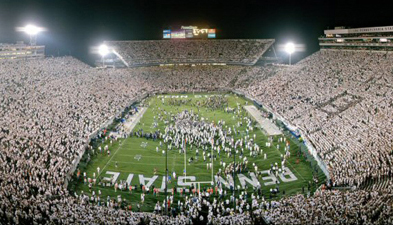
Select three fans randomly at a football game in which Penn State is playing Notre Dame. Identify whether the fan is a Penn State fan (\(P\)) or a Notre Dame fan (\(N\)). This experiment yields the following sample space:
\(\mathbf{S}=\{PPP, PPN, PNP, NPP, NNP, NPN, PNN, NNN\}\)
Let \(X\) = the number of Penn State fans selected. The possible values of \(X\) are, therefore, either 0, 1, 2, or 3. Now, we could find probabilities of individual events, \(P(PPP)\) or \(P(PPN)\), for example. Alternatively, we could find \(P(X=x)\), the probability that \(X\) takes on a particular value \(x\). Let's do that!
Since the game is a home game, let's suppose that 80% of the fans attending the game are Penn State fans, while 20% are Notre Dame fans. That is, \(P(P)=0.8\) and \(P(N)=0.2\). Then, by independence:
\(P(X=0)=P(NNN)=0.2\times0.2\times0.2=0.008\)
And, by independence and mutual exclusivity of \(NNP, NPN\), and \(PNN\):
\(P(X=1)=P(NNP)+P(NPN)+P(PNN)=3\times0.2\times0.2\times0.8=0.096\)
Likewise, by independence and mutual exclusivity of \(PPN, PNP\), and \(NPP\):
\(P(X=2)=P(PPN)+P(PNP)+P(NPP)=3\times0.8\times0.8\times0.2=0.384\)
Finally, by independence:
\(P(X = 3) = P(PPP) = 0.8\times0.8\times0.8 = 0.512\)
There are a few things to note here:
- The results make sense! Given that 80% of the fans in the stands are Penn State fans, it shouldn't seem surprising that we would be most likely to select 2 or 3 Penn State fans.
- The probabilities behave well in that (1) the probabilities are all greater than 0, that is, \(P(X=x)>0\) and (2) the probability of the sample space is 1, that is,\(P(\mathbf{S}) = P(X = 0) + P(X = 1) + P(X = 2) + P(X = 3) = 1\).
- Because the values that it takes on are random, the variable \(X\) has a special name. It is called a random variable! Ta-daaaa!
Let's give a formal definition of a random variable.
- Random Variable \(X\)
-
Given a random experiment with sample space \(\mathbf{S}\),a random variable \(X\) is a set function that assigns one and only one real number to each element \(s\) that belongs in the sample space \(\mathbf{S}\).
The set of all possible values of the random variable \(X\),denoted \(x\),is called the support, or space, of \(X\).
Note that the capital letters at the end of the alphabet, such as \(W, X, Y\), and \(Z\) typically represent the definition of the random variable. The corresponding lowercase letters, such as \(w, x, y\), and \(z\), represent the random variable's possible values.
Example 7-2
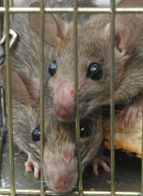
A rat is selected at random from a cage of male (\(M\)) and female rats (\(F\)). Once selected, the gender of the selected rat is noted. The sample space is thus:
\(\mathbf{S} = \{M, F\}\)
Define the random variable \(X\) as follows:
- Let \(X = 0\) if the rat is male.
- Let \(X = 1\) if the rat is female.
Note that the random variable \(X\) assigns one and only one real number (0 and 1) to each element of the sample space (\(M\) and \(F\)). The support, or space, of \(X\) is \(\{0, 1\}\).
Note that we don't necessarily need to use the numbers 0 and 1 as the support. For example, we could have alternatively (and perhaps arbitrarily?!) used the numbers 5 and 15, respectively. In that case, our random variable would be defined as \(X = 5\) of the rat is male, and \(X = 15\) if the rat is female.
Example 7-3
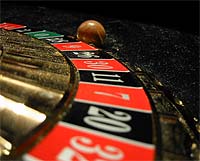
A roulette wheel has 38 numbers on it: a zero (0), a double zero (00), and the numbers 1, 2, 3, ..., 36. Spin the wheel until the pointer lands on number 36. One possibility is that the wheel lands on 36 on the first spin. Another possibility is that the wheel lands on 0 on the first spin, and 36 on the second spin. Yet another possibility is that the wheel lands on 0 on the first spin, 7 on the second spin, and 36 on the third spin. The sample space must list all of the countably infinite (!) number of possible sequences. That is, the sample space looks like this:
\(\mathbf{S} = \{36, 0-36, 00-36, 1-36, \ldots, 35-36, 0-0-36, 0-1-36, \ldots\}\)
If we define the random variable \(X\) to equal the number of spins until the wheel lands on 36, then the support of \(X\) is \(\{0, 1, 2, 3, \ldots\}\).
Note that in the rat example, there were a finite (two, to be exact) number of possible outcomes, while in the roulette example, there were a countably infinite number of possible outcomes. This leads us to the following formal definition.
- Discrete Random Variable
-
A random variable \(X\) is a discrete random variable if:
- there are a finite number of possible outcomes of \(X\), or
- there are a countably infinite number of possible outcomes of \(X\).
Recall that a countably infinite number of possible outcomes means that there is a one-to-one correspondence between the outcomes and the set of integers. No such one-to-one correspondence exists for an uncountably infinite number of possible outcomes.
As you might have guessed by its name, we will be studying discrete random variables and their probability distributions throughout Section 2.
7.2 - Probability Mass Functions
7.2 - Probability Mass FunctionsThe probability that a discrete random variable \(X\) takes on a particular value \(x\), that is, \(P(X = x)\), is frequently denoted \(f(x)\). The function \(f(x)\) is typically called the probability mass function, although some authors also refer to it as the probability function, the frequency function, or probability density function. We will use the common terminology — the probability mass function — and its common abbreviation —the p.m.f.
- Probability Mass Function
-
The probability mass function, \(P(X=x)=f(x)\), of a discrete random variable \(X\) is a function that satisfies the following properties:
- \(P(X=x)=f(x)>0\), if \(x\in \text{ the support }S\)
- \(\sum\limits_{x\in S} f(x)=1\)
- \(P(X\in A)=\sum\limits_{x\in A} f(x)\)
First item basically says that, for every element \(x\) in the support \(S\), all of the probabilities must be positive. Note that if \(x\) does not belong in the support \(S\), then \(f(x) = 0\). The second item basically says that if you add up the probabilities for all of the possible \(x\) values in the support \(S\), then the sum must equal 1. And, the third item says to determine the probability associated with the event \(A\), you just sum up the probabilities of the \(x\) values in \(A\).
Since \(f(x)\) is a function, it can be presented:
- in tabular form
- in graphical form
- as a formula
Let's take a look at a few examples.
Example 7-4
Let \(X\) equal the number of siblings of Penn State students. The support of \(X\) is, of course, 0, 1, 2, 3, ... Because the support contains a countably infinite number of possible values, \(X\) is a discrete random variable with a probability mass function. Find \(f(x) = P(X = x)\), the probability mass function of \(X\), for all \(x\) in the support.
This example illustrated the tabular and graphical forms of a p.m.f. Now let's take a look at an example of a p.m.f. in functional form.
Example 7-5
Let \(f(x)=cx^2\) for \(x = 1, 2, 3\). Determine the constant \(c\) so that the function \(f(x)\) satisfies the conditions of being a probability mass function.
Answer
The key to finding \(c\) is to use item #2 in the definition of a p.m.f.
The support in this example is finite. Let's take a look at an example in which the support is countably infinite.
Example 7-6
Determine the constant \(c\) so that the following p.m.f. of the random variable \(Y\) is a valid probability mass function:
\(f(y)=c\left(\dfrac{1}{4}\right)^y\) for y = 1, 2, 3, ...
Answer
Again, the key to finding \(c\) is to use item #2 in the definition of a p.m.f.
7.3 - The Cumulative Distribution Function (CDF)
7.3 - The Cumulative Distribution Function (CDF)The cumulative distribution function (CDF or cdf) of the random variable \(X\) has the following definition:
\(F_X(t)=P(X\le t)\)
The cdf is discussed in the text as well as in the notes but I wanted to point out a few things about this function. The cdf is not discussed in detail until section 2.4 but I feel that introducing it earlier is better. The notation sometimes confuses students. The notation \(F_X(t)\) means that \(F\) is the cdf for the random variable \(X\) but it is a function of \(t\).
We do not focus too much on the cdf for a discrete random variable but we will use them very often when we study continuous random variables. It does not mean that the cdf is not important for discrete random variables. They are just not always used since there are tables and software that help us to find these probabilities for common distributions.
The cdf of random variable \(X\) has the following properties:
- \(F_X(t)\) is a nondecreasing function of \(t\), for \(-\infty<t<\infty\).
- The cdf, \(F_X(t)\), ranges from 0 to 1. This makes sense since \(F_X(t)\) is a probability.
- If \(X\) is a discrete random variable whose minimum value is \(a\), then \(F_X(a)=P(X\le a)=P(X=a)=f_X(a)\). If \(c\) is less than \(a\), then \(F_X(c)=0\).
- If the maximum value of \(X\) is \(b\), then \(F_X(b)=1\).
- Also called the distribution function.
- All probabilities concerning \(X\) can be stated in terms of \(F\).
I have provided a few very brief examples using the cdf. We will be looking at these functions in more detail in the future.
Suppose \(X\) is a discrete random variable. Let the pmf of \(X\) be equal to
\(f(x)=\dfrac{5-x}{10}, \;\; x=1,2,3,4.\)
Suppose we want to find the cdf of \(X\). The cdf is \(F_X(t)=P(X\le t)\).
- For \(t=1\), \(P(X\le 1)=P(X=1)=f(1)=\dfrac{5-1}{10}=\dfrac{4}{10}\).
- For \(t=2\), \(P(X\le 2)=P(X=1 \text{ or } X=2)=P(X=1)+P(X=2)=\dfrac{5-1}{10}+\dfrac{5-2}{10}=\dfrac{4+3}{10}=\dfrac{7}{10}\)
- For \(t=3\), \(P(X\le 3)=\dfrac{5-1}{10}+\dfrac{5-2}{10}+\dfrac{5-3}{10}=\dfrac{4+3+1}{10}=\dfrac{9}{10}\).
- For \(t=4\), \(P(X\le 4)=\dfrac{5-1}{10}+\dfrac{5-2}{10}+\dfrac{5-3}{10}+\dfrac{5-4}{10}=\dfrac{10}{10}=1\).
It is worth noting that \(P(X\le 2)\) does not equal \(P(X<2)\); \(P(X\le 2)=P(X=1, 2)\) and \(P(X<2)=P(X=1)\). It is very important for you to carefully read the problems in order to correctly set up the probabilities. You should also look carefully at the notation if a problem provides it.
Consider \(X\) to be a random variable (a binomial random variable) with the following pmf
\(f(x)=P(X=x)={n\choose x}p^x(1-p)^{n-x}, \;\; \text{for } x=0, 1, \cdots , n.\)
The cdf of \(X\) evaluated at \(t\), denoted \(F_X(t)\), is
\(F_X(t)=\sum_{x=0}^t {n\choose x}p^x(1-p)^{n-x}, \;\; \text{for } 0\le t\le n.\)
- When \(t=0\), we have \(F_X(0)={n\choose 0}p^0(1-p)^{n-0}\).
- When \(t=1\), we have \(F_X(1)={n\choose 0}p^0(1-p)^{n-0}+{n\choose 1}p^1(1-p)^{n-1}\).
- When \(t=2\), we have \(F_X(2)={n\choose 0}p^0(1-p)^{n-0}+{n\choose 1}p^1(1-p)^{n-1}+ {n\choose 2}p^2(1-p)^{n-2}\).
And so on and so forth.
One last example. Suppose we have a family with three children. The sample space for this situation is
\(\mathbf{S}= \left \{ BBB, BBG, BGB, GBB, GGG, GGB, GBG, BGG \right \} \)
where \(B\) = boy and \(G\) = girl and suppose the probability of having a boy is the same as the probability of having a girl. Let the random variable \(X\) be the number of boys. Then \(X\) will have the following pmf:
| t | 0 | 1 | 2 | 3 |
| \(P(X=t)\) | \(\dfrac{1}{8}\) | \(\dfrac{3}{8}\) | \(\dfrac{3}{8}\) | \(\dfrac{1}{8}\) |
Then, we can use the pmf to find the cdf.
| t | 0 | 1 | 2 | 3 |
| \(F_X(t)=P(X\le t)\) | \(\dfrac{1}{8}\) | \(\dfrac{1}{8}+\dfrac{3}{8}=\dfrac{4}{8}\) | \(\dfrac{4}{8}+\dfrac{3}{8}=\dfrac{7}{8}\) | \(\dfrac{7}{8}+\dfrac{1}{8}=1\) |
Additional Practice Problem
These are some theoretical problems for the CDF and for expectations. Work these problems out on your own and then click on the link to view the solution.
- Express the following probabilities in terms of the cdf, \(F_X(t)\), if \(X\) is a discrete random variable with support such that \(x\) being any integer from 0 to \(b\) and \(0\le a\le b\):
-
\(P(X\le a)\)\(P(X\le a)=F_X(a)\) by definition of cdf
-
\(f_X(a)=P(X=a)\), where \(f_X(x)\) is the pmf of \(X\)\(P(X=a)=P(X\le a)-P(X\le a-1)=F_X(a)-F_X(a-1)\)
-
\(P(X<a)\)\(P(X<a)=P(X\le a)-P(X=a)=P(X\le a-1)=F_X(a-1)\)
-
\(P(X\ge a)\)\(P(X\ge a)=1-P(X\le a-1)=1-F_X(a-1)\)
-
-
Let \(X\) have distribution function \(F\). What is the distribution function and expectation of \(\dfrac{X - \mu}{\sigma}\)? In other words, find the distribution function in terms of \(F_X\) and the expectation in terms of \(E(X)\).
Let \(Y=\dfrac{X-\mu}{\sigma}\). We want \(F_Y(t)\) and \(E(Y)\).
\begin{align*} & F_Y(y)=P(Y\le y), \text{ by definition of cdf of Y}\\ & F_Y(y)=P(Y\le y)=P\left(\dfrac{X-\mu}{\sigma}\le y\right)=P\left(X\le y\sigma+\mu\right)\\ & F_Y(y)= F_X(t\sigma+\mu) \end{align*}
Now, to find the expectation, we can do this in two ways. One way is to find it using the definition of expectation, \(E(Y)=\sum_y yf_Y(y)\). In order to do this though, we would need to find \(f_Y(y)\), which we can find using the CDF if \(F_X\) was given.
The other way to approach this is to use the properties of expectation.
\(E(Y)=E\left(\dfrac{X-\mu}{\sigma}\right)=\dfrac{1}{\sigma}E(X-\mu)=\dfrac{E(X)-\mu}{\sigma}\)
7.4 - Hypergeometric Distribution
7.4 - Hypergeometric DistributionExample 7-7

A crate contains 50 light bulbs of which 5 are defective and 45 are not. A Quality Control Inspector randomly samples 4 bulbs without replacement. Let \(X\) = the number of defective bulbs selected. Find the probability mass function, \(f(x)\), of the discrete random variable \(X\).
This example is an example of a random variable \(X\) following what is called the hypergeometric distribution. Let's generalize our findings.
- Hypergeometric distribution
-
If we randomly select \(n\) items without replacement from a set of \(N\) items of which:
\(m\) of the items are of one type and \(N-m\) of the items are of a second typethen the probability mass function of the discrete random variable \(X\) is called the hypergeometric distribution and is of the form:
\(P(X=x)=f(x)=\dfrac{\dbinom{m}{x} \dbinom{N-m}{n-x}}{\dbinom{N}{n}}\)
where the support \(S\) is the collection of nonnegative integers x that satisfies the inequalities:
\(x\le n\) \(x\le m\) \(n-x\le N-m\)
Note that one of the key features of the hypergeometric distribution is that it is associated with sampling without replacement. We will see later, in Lesson 9, that when the samples are drawn with replacement, the discrete random variable \(X\) follows what is called the binomial distribution.
7.5 - More Examples
7.5 - More ExamplesExample 7-8
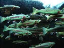
A lake contains 600 fish, eighty (80) of which have been tagged by scientists. A researcher randomly catches 15 fish from the lake. Find a formula for the probability mass function of \(X\), the number of fish in the researcher's sample which are tagged.
Solution
This problem is very similar to the example on the previous page in which we were interested in finding the p.m.f. of \(X\), the number of defective bulbs selected in a sample of 4 bulbs. Here, we are interested in finding \(X\), the number of tagged fish selected in a sample of 15 fish. That is, \(X\) is a hypergeometric random variable with \(m = 80\), \(N = 600\), and \(n = 15\). Therefore, the p.m.f. of \(X\) is:
for the support \(x=0, 1, 2, \ldots, 15\).
Example 7-9
Let the random variable \(X\) denote the number of aces in a five-card hand dealt from a standard 52-card deck. Find a formula for the probability mass function of \(X\).
Solution
The random variable \(X\) here also follows the hypergeometric distribution. Here, there are \(N=52\) total cards, \(n=5\) cards sampled, and \(m=4\) aces. Therefore, the p.m.f. of \(X\) is:
\(f(x)=\dfrac{\dbinom{4}{x} \dbinom{48}{5-x}}{\dbinom{52}{5}}\)
for the support \(x=0, 1, 2, 3, 4\).
Example 7-10

Suppose that 5 people, including you and a friend, line up at random. Let the random variable \(X\) denote the number of people standing between you and a friend. Determine the probability mass function of \(X\) in tabular form. Also, verify that the p.m.f. is a valid p.m.f.