7.1 - Discrete Random Variables
7.1 - Discrete Random VariablesExample 7-1

Select three fans randomly at a football game in which Penn State is playing Notre Dame. Identify whether the fan is a Penn State fan (\(P\)) or a Notre Dame fan (\(N\)). This experiment yields the following sample space:
\(\mathbf{S}=\{PPP, PPN, PNP, NPP, NNP, NPN, PNN, NNN\}\)
Let \(X\) = the number of Penn State fans selected. The possible values of \(X\) are, therefore, either 0, 1, 2, or 3. Now, we could find probabilities of individual events, \(P(PPP)\) or \(P(PPN)\), for example. Alternatively, we could find \(P(X=x)\), the probability that \(X\) takes on a particular value \(x\). Let's do that!
Since the game is a home game, let's suppose that 80% of the fans attending the game are Penn State fans, while 20% are Notre Dame fans. That is, \(P(P)=0.8\) and \(P(N)=0.2\). Then, by independence:
\(P(X=0)=P(NNN)=0.2\times0.2\times0.2=0.008\)
And, by independence and mutual exclusivity of \(NNP, NPN\), and \(PNN\):
\(P(X=1)=P(NNP)+P(NPN)+P(PNN)=3\times0.2\times0.2\times0.8=0.096\)
Likewise, by independence and mutual exclusivity of \(PPN, PNP\), and \(NPP\):
\(P(X=2)=P(PPN)+P(PNP)+P(NPP)=3\times0.8\times0.8\times0.2=0.384\)
Finally, by independence:
\(P(X = 3) = P(PPP) = 0.8\times0.8\times0.8 = 0.512\)
There are a few things to note here:
- The results make sense! Given that 80% of the fans in the stands are Penn State fans, it shouldn't seem surprising that we would be most likely to select 2 or 3 Penn State fans.
- The probabilities behave well in that (1) the probabilities are all greater than 0, that is, \(P(X=x)>0\) and (2) the probability of the sample space is 1, that is,\(P(\mathbf{S}) = P(X = 0) + P(X = 1) + P(X = 2) + P(X = 3) = 1\).
- Because the values that it takes on are random, the variable \(X\) has a special name. It is called a random variable! Ta-daaaa!
Let's give a formal definition of a random variable.
- Random Variable \(X\)
-
Given a random experiment with sample space \(\mathbf{S}\),a random variable \(X\) is a set function that assigns one and only one real number to each element \(s\) that belongs in the sample space \(\mathbf{S}\).
The set of all possible values of the random variable \(X\),denoted \(x\),is called the support, or space, of \(X\).
Note that the capital letters at the end of the alphabet, such as \(W, X, Y\), and \(Z\) typically represent the definition of the random variable. The corresponding lowercase letters, such as \(w, x, y\), and \(z\), represent the random variable's possible values.
Example 7-2

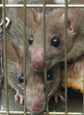
A rat is selected at random from a cage of male (\(M\)) and female rats (\(F\)). Once selected, the gender of the selected rat is noted. The sample space is thus:
\(\mathbf{S} = \{M, F\}\)
Define the random variable \(X\) as follows:
- Let \(X = 0\) if the rat is male.
- Let \(X = 1\) if the rat is female.
Note that the random variable \(X\) assigns one and only one real number (0 and 1) to each element of the sample space (\(M\) and \(F\)). The support, or space, of \(X\) is \(\{0, 1\}\).
Note that we don't necessarily need to use the numbers 0 and 1 as the support. For example, we could have alternatively (and perhaps arbitrarily?!) used the numbers 5 and 15, respectively. In that case, our random variable would be defined as \(X = 5\) of the rat is male, and \(X = 15\) if the rat is female.
Example 7-3

A roulette wheel has 38 numbers on it: a zero (0), a double zero (00), and the numbers 1, 2, 3, ..., 36. Spin the wheel until the pointer lands on number 36. One possibility is that the wheel lands on 36 on the first spin. Another possibility is that the wheel lands on 0 on the first spin, and 36 on the second spin. Yet another possibility is that the wheel lands on 0 on the first spin, 7 on the second spin, and 36 on the third spin. The sample space must list all of the countably infinite (!) number of possible sequences. That is, the sample space looks like this:
\(\mathbf{S} = \{36, 0-36, 00-36, 1-36, \ldots, 35-36, 0-0-36, 0-1-36, \ldots\}\)
If we define the random variable \(X\) to equal the number of spins until the wheel lands on 36, then the support of \(X\) is \(\{0, 1, 2, 3, \ldots\}\).
Note that in the rat example, there were a finite (two, to be exact) number of possible outcomes, while in the roulette example, there were a countably infinite number of possible outcomes. This leads us to the following formal definition.
- Discrete Random Variable
-
A random variable \(X\) is a discrete random variable if:
- there are a finite number of possible outcomes of \(X\), or
- there are a countably infinite number of possible outcomes of \(X\).
Recall that a countably infinite number of possible outcomes means that there is a one-to-one correspondence between the outcomes and the set of integers. No such one-to-one correspondence exists for an uncountably infinite number of possible outcomes.
As you might have guessed by its name, we will be studying discrete random variables and their probability distributions throughout Section 2.