Lesson 26: Random Functions Associated with Normal Distributions
Lesson 26: Random Functions Associated with Normal DistributionsOverview
In the previous lessons, we've been working our way up towards fully defining the probability distribution of the sample mean \(\bar{X}\) and the sample variance \(S^2\). We have determined the expected value and variance of the sample mean. Now, in this lesson, we (finally) determine the probability distribution of the sample mean and sample variance when a random sample \(X_1, X_2, \ldots, X_n\) is taken from a normal population (distribution). We'll also learn about a new probability distribution called the (Student's) t distribution.
Objectives
- To learn the probability distribution of a linear combination of independent normal random variables \(X_1, X_2, \ldots, X_n\).
- To learn how to find the probability that a linear combination of independent normal random variables \(X_1, X_2, \ldots, X_n\) takes on a certain interval of values.
- To learn the sampling distribution of the sample mean when \(X_1, X_2, \ldots, X_n\) are a random sample from a normal population with mean \(\mu\) and variance \(\sigma^2\).
- To use simulation to get a feel for the shape of a probability distribution.
- To learn the sampling distribution of the sample variance when \(X_1, X_2, \ldots, X_n\) are a random sample from a normal population with mean \(\mu\) and variance \(\sigma^2\).
- To learn the formal definition of a \(T\) random variable.
- To learn the characteristics of Student's \(t\) distribution.
- To learn how to read a \(t\)-table to find \(t\)-values and probabilities associated with \(t\)-values.
- To understand each of the steps in the proofs in the lesson.
- To be able to apply the methods learned in this lesson to new problems.
26.1 - Sums of Independent Normal Random Variables
26.1 - Sums of Independent Normal Random VariablesWell, we know that one of our goals for this lesson is to find the probability distribution of the sample mean when a random sample is taken from a population whose measurements are normally distributed. Then, let's just get right to the punch line! Well, first we'll work on the probability distribution of a linear combination of independent normal random variables \(X_1, X_2, \ldots, X_n\). On the next page, we'll tackle the sample mean!
If \(X_1, X_2, \ldots, X_n\) >are mutually independent normal random variables with means \(\mu_1, \mu_2, \ldots, \mu_n\) and variances \(\sigma^2_1,\sigma^2_2,\cdots,\sigma^2_n\), then the linear combination:
\(Y=\sum\limits_{i=1}^n c_iX_i\)
follows the normal distribution:
\(N\left(\sum\limits_{i=1}^n c_i \mu_i,\sum\limits_{i=1}^n c^2_i \sigma^2_i\right)\)
Proof
We'll use the moment-generating function technique to find the distribution of \(Y\). In the previous lesson, we learned that the moment-generating function of a linear combination of independent random variables \(X_1, X_2, \ldots, X_n\) >is:
\(M_Y(t)=\prod\limits_{i=1}^n M_{X_i}(c_it)\)
Now, recall that if \(X_i\sim N(\mu, \sigma^2)\), then the moment-generating function of \(X_i\) is:
\(M_{X_i}(t)=\text{exp} \left(\mu t+\dfrac{\sigma^2t^2}{2}\right)\)
Therefore, the moment-generating function of \(Y\) is:
\(M_Y(t)=\prod\limits_{i=1}^n M_{X_i}(c_it)=\prod\limits_{i=1}^n \text{exp} \left[\mu_i(c_it)+\dfrac{\sigma^2_i(c_it)^2}{2}\right] \)
Evaluating the product at each index \(i\) from 1 to \(n\), and using what we know about exponents, we get:
\(M_Y(t)=\text{exp}(\mu_1c_1t) \cdot \text{exp}(\mu_2c_2t) \cdots \text{exp}(\mu_nc_nt) \cdot \text{exp}\left(\dfrac{\sigma^2_1c^2_1t^2}{2}\right) \cdot \text{exp}\left(\dfrac{\sigma^2_2c^2_2t^2}{2}\right) \cdots \text{exp}\left(\dfrac{\sigma^2_nc^2_nt^2}{2}\right) \)
Again, using what we know about exponents, and rewriting what we have using summation notation, we get:
\(M_Y(t)=\text{exp}\left[t\left(\sum\limits_{i=1}^n c_i \mu_i\right)+\dfrac{t^2}{2}\left(\sum\limits_{i=1}^n c^2_i \sigma^2_i\right)\right]\)
Ahaaa! We have just shown that the moment-generating function of \(Y\) is the same as the moment-generating function of a normal random variable with mean:
\(\sum\limits_{i=1}^n c_i \mu_i\)
and variance:
\(\sum\limits_{i=1}^n c^2_i \sigma^2_i\)
Therefore, by the uniqueness property of moment-generating functions, \(Y\) must be normally distributed with the said mean and said variance. Our proof is complete.
Example 26-1
Let \(X_1\) be a normal random variable with mean 2 and variance 3, and let \(X_2\) be a normal random variable with mean 1 and variance 4. Assume that \(X_1\) and \(X_2\) are independent. What is the distribution of the linear combination \(Y=2X_1+3X_2\)?
Solution
The previous theorem tells us that \(Y\) is normally distributed with mean 7 and variance 48 as the following calculation illustrates:
\((2X_1+3X_2)\sim N(2(2)+3(1),2^2(3)+3^2(4))=N(7,48)\)
What is the distribution of the linear combination \(Y=X_1-X_2\)?
Solution
The previous theorem tells us that \(Y\) is normally distributed with mean 1 and variance 7 as the following calculation illustrates:
\((X_1-X_2)\sim N(2-1,(1)^2(3)+(-1)^2(4))=N(1,7)\)
Example 26-2
History suggests that scores on the Math portion of the Standard Achievement Test (SAT) are normally distributed with a mean of 529 and a variance of 5732. History also suggests that scores on the Verbal portion of the SAT are normally distributed with a mean of 474 and a variance of 6368. Select two students at random. Let \(X\) denote the first student's Math score, and let \(Y\) denote the second student's Verbal score. What is \(P(X>Y)\)?
Solution
We can find the requested probability by noting that \(P(X>Y)=P(X-Y>0)\), and then taking advantage of what we know about the distribution of \(X-Y\). That is, \(X-Y\) is normally distributed with a mean of 55 and variance of 12100 as the following calculation illustrates:
\((X-Y)\sim N(529-474,(1)^2(5732)+(-1)^2(6368))=N(55,12100)\)
Then, finding the probability that \(X\) is greater than \(Y\) reduces to a normal probability calculation:
\begin{align} P(X>Y) &=P(X-Y>0)\\ &= P\left(Z>\dfrac{0-55}{\sqrt{12100}}\right)\\ &= P\left(Z>-\dfrac{1}{2}\right)=P\left(Z<\dfrac{1}{2}\right)=0.6915\\ \end{align}
That is, the probability that the first student's Math score is greater than the second student's Verbal score is 0.6915.
Example 26-3
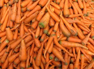
Let \(X_i\) denote the weight of a randomly selected prepackaged one-pound bag of carrots. Of course, one-pound bags of carrots won't weigh exactly one pound. In fact, history suggests that \(X_i\) is normally distributed with a mean of 1.18 pounds and a standard deviation of 0.07 pound.
Now, let \(W\) denote the weight of randomly selected prepackaged three-pound bag of carrots. Three-pound bags of carrots won't weigh exactly three pounds either. In fact, history suggests that \(W\) is normally distributed with a mean of 3.22 pounds and a standard deviation of 0.09 pound.
Selecting bags at random, what is the probability that the sum of three one-pound bags exceeds the weight of one three-pound bag?
Solution
Because the bags are selected at random, we can assume that \(X_1, X_2, X_3\) and \(W\) are mutually independent. The theorem helps us determine the distribution of \(Y\), the sum of three one-pound bags:
\(Y=(X_1+X_2+X_3) \sim N(1.18+1.18+1.18, 0.07^2+0.07^2+0.07^2)=N(3.54,0.0147)\)
That is, \(Y\) is normally distributed with a mean of 3.54 pounds and a variance of 0.0147. Now, \(Y-W\), the difference in the weight of three one-pound bags and one three-pound bag is normally distributed with a mean of 0.32 and a variance of 0.0228, as the following calculation suggests:
\((Y-W) \sim N(3.54-3.22,(1)^2(0.0147)+(-1)^2(0.09^2))=N(0.32,0.0228)\)
Therefore, finding the probability that \(Y\) is greater than \(W\) reduces to a normal probability calculation:
\begin{align} P(Y>W) &=P(Y-W>0)\\ &= P\left(Z>\dfrac{0-0.32}{\sqrt{0.0228}}\right)\\ &= P(Z>-2.12)=P(Z<2.12)=0.9830\\ \end{align}
That is, the probability that the sum of three one-pound bags exceeds the weight of one three-pound bag is 0.9830. Hey, if you want more bang for your buck, it looks like you should buy multiple one-pound bags of carrots, as opposed to one three-pound bag!
26.2 - Sampling Distribution of Sample Mean
26.2 - Sampling Distribution of Sample MeanOkay, we finally tackle the probability distribution (also known as the "sampling distribution") of the sample mean when \(X_1, X_2, \ldots, X_n\) are a random sample from a normal population with mean \(\mu\) and variance \(\sigma^2\). The word "tackle" is probably not the right choice of word, because the result follows quite easily from the previous theorem, as stated in the following corollary.
If \(X_1, X_2, \ldots, X_n\) are observations of a random sample of size \(n\) from a \(N(\mu, \sigma^2)\) population, then the sample mean:
\(\bar{X}=\dfrac{1}{n}\sum\limits_{i=1}^n X_i\)
is normally distributed with mean \(\mu\) and variance \(\frac{\sigma^2}{n}\). That is, the probability distribution of the sample mean is:
\(N(\mu,\sigma^2/n)\)
Proof
The result follows directly from the previous theorem. All we need to do is recognize that the sample mean:
\(\bar{X}=\dfrac{X_1+X_2+\cdots+X_n}{n}\)
is a linear combination of independent normal random variables:
\(\bar{X}=\dfrac{1}{n} X_1+\dfrac{1}{n} X_2+\cdots+\dfrac{1}{n} X_n\)
with \(c_i=\frac{1}{n}\), the mean \(\mu_i=\mu\) and the variance \(\sigma^2_i=\sigma^2\). That is, the moment generating function of the sample mean is then:
\(M_{\bar{X}}(t)=\text{exp}\left[t\left(\sum\limits_{i=1}^n c_i \mu_i\right)+\dfrac{t^2}{2}\left(\sum\limits_{i=1}^n c^2_i \sigma^2_i\right)\right]=\text{exp}\left[t\left(\sum\limits_{i=1}^n \dfrac{1}{n}\mu\right)+\dfrac{t^2}{2}\left(\sum\limits_{i=1}^n \left(\dfrac{1}{n}\right)^2\sigma^2\right)\right]\)
The first equality comes from the theorem on the previous page, about the distribution of a linear combination of independent normal random variables. The second equality comes from simply replacing \(c_i\) with \(\frac{1}{n}\), the mean \(\mu_i\) with \(\mu\) and the variance \(\sigma^2_i\) with \(\sigma^2\). Now, working on the summations, the moment generating function of the sample mean reduces to:
\(M_{\bar{X}}(t)=\text{exp}\left[t\left(\dfrac{1}{n} \sum\limits_{i=1}^n \mu\right)+\dfrac{t^2}{2}\left(\dfrac{1}{n^2}\sum\limits_{i=1}^n \sigma^2\right)\right]=\text{exp}\left[t\left(\dfrac{1}{n}(n\mu)\right)+\dfrac{t^2}{2}\left(\dfrac{1}{n^2}(n\sigma^2)\right)\right]=\text{exp}\left[\mu t +\dfrac{t^2}{2} \left(\dfrac{\sigma^2}{n}\right)\right]\)
The first equality comes from pulling the constants depending on \(n\) through the summation signs. The second equality comes from adding \(\mu\) up \(n\) times to get \(n\mu\), and adding \(\sigma^2\) up \(n\) times to get \(n\sigma^2\). The last equality comes from simplifying a bit more. In summary, we have shown that the moment generating function of the sample mean of \(n\) independent normal random variables with mean \(\mu\) and variance \(\sigma^2\) is:
\(M_{\bar{X}}(t)=\text{exp}\left[\mu t +\dfrac{t^2}{2} \left(\dfrac{\sigma^2}{n}\right)\right]\)
That is the same as the moment generating function of a normal random variable with mean \(\mu\) and variance \(\frac{\sigma^2}{n}\). Therefore, the uniqueness property of moment-generating functions tells us that the sample mean must be normally distributed with mean \(\mu\) and variance \(\frac{\sigma^2}{n}\). Our proof is complete.
Example 26-4
Let \(X_i\) denote the Stanford-Binet Intelligence Quotient (IQ) of a randomly selected individual, \(i=1, \ldots, 4\) (one sample). Let \(Y_i\) denote the IQ of a randomly selected individual, \(i=1, \ldots, 8\) (a second sample). Recalling that IQs are normally distributed with mean \(\mu=100\) and variance \(\sigma^2=16^2\), what is the distribution of \(\bar{X}\)? And, what is the distribution of \(\bar{Y}\)?
Anwser
In general, the variance of the sample mean is:
\(Var(\bar{X})=\dfrac{\sigma^2}{n}\)
Therefore, the variance of the sample mean of the first sample is:
\(Var(\bar{X}_4)=\dfrac{16^2}{4}=64\)
(The subscript 4 is there just to remind us that the sample mean is based on a sample of size 4.) And, the variance of the sample mean of the second sample is:
\(Var(\bar{Y}_8=\dfrac{16^2}{8}=32\)
(The subscript 8 is there just to remind us that the sample mean is based on a sample of size 8.) Now, the corollary therefore tells us that the sample mean of the first sample is normally distributed with mean 100 and variance 64. That is:
\(\bar{X}_4 \sim N(100,64)\)
And, the sample mean of the second sample is normally distributed with mean 100 and variance 32. That is:
\(\bar{Y}_8 \sim N(100,32)\)
So, we have two, no actually, three normal random variables with the same mean, but difference variances:
- We have \(X_i\), an IQ of a random individual. It is normally distributed with mean 100 and variance 256.
- We have \(\bar{X}_4\), the average IQ of 4 random individuals. It is normally distributed with mean 100 and variance 64.
- We have \(\bar{Y}_8\), the average IQ of 8 random individuals. It is normally distributed with mean 100 and variance 32.
It is quite informative to graph these three distributions on the same plot. Doing so, we get:
As the plot suggests, an individual \(X_i\), the mean (\bar{X}_4\) and the mean \(\bar{Y}_8\) all provide valid, "unbiased" estimates of the population mean \(\mu\). But, our intuition coincides with reality... that is, the sample mean \(\bar{Y}_8\) will be the most precise estimate of \(\mu\).
All the work that we have done so far concerning this example has been theoretical in nature. That is, what we have learned is based on probability theory. Would we see the same kind of result if we were take to a large number of samples, say 1000, of size 4 and 8, and calculate the sample mean of each sample? That is, would the distribution of the 1000 sample means based on a sample of size 4 look like a normal distribution with mean 100 and variance 64? And would the distribution of the 1000 sample means based on a sample of size 8 look like a normal distribution with mean 100 and variance 32? Well, the only way to answer these questions is to try it out!
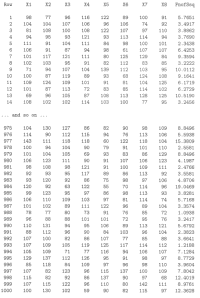
I did just that for us. I used Minitab to generate 1000 samples of eight random numbers from a normal distribution with mean 100 and variance 256. Here's a subset of the resulting random numbers:
| ROW | X1 | X2 | X3 | X4 | X5 | X6 | X7 | X8 | Mean 4 | Mean 8 |
| 1 | 87 | 68 | 98 | 114 | 59 | 111 | 114 | 86 | 91.75 | 92.125 |
| 2 | 102 | 81 | 74 | 110 | 112 | 106 | 105 | 99 | 91.75 | 98.625 |
| 3 | 96 | 87 | 50 | 88 | 69 | 107 | 94 | 83 | 80.25 | 84.250 |
| 4 | 83 | 134 | 122 | 80 | 117 | 110 | 115 | 158 | 104.75 | 114.875 |
| 5 | 92 | 87 | 120 | 93 | 90 | 111 | 95 | 92 | 98.00 | 97.500 |
| 6 | 139 | 102 | 100 | 103 | 111 | 62 | 78 | 73 | 111.00 | 96.000 |
| 7 | 134 | 121 | 99 | 118 | 108 | 106 | 103 | 91 | 118.00 | 110.000 |
| 8 | 126 | 92 | 148 | 131 | 99 | 106 | 143 | 128 | 124.25 | 121.625 |
| 9 | 98 | 109 | 119 | 110 | 124 | 99 | 119 | 82 | 109.00 | 107.500 |
| 10 | 85 | 93 | 82 | 106 | 93 | 109 | 100 | 95 | 91.50 | 95.375 |
| 11 | 121 | 103 | 108 | 96 | 112 | 117 | 93 | 112 | 107.00 | 107.750 |
| 12 | 118 | 91 | 106 | 108 | 128 | 96 | 65 | 85 | 105.75 | 99.625 |
| 13 | 92 | 87 | 96 | 81 | 86 | 105 | 91 | 104 | 89.00 | 92.750 |
| 14 | 94 | 115 | 59 | 105 | 101 | 122 | 97 | 103 | 93.25 | 99.500 |
| ...and so on... | ||||||||||
| 975 | 108 | 139 | 130 | 97 | 138 | 88 | 104 | 87 | 118.50 | 111.375 |
| 976 | 99 | 122 | 93 | 107 | 98 | 62 | 102 | 115 | 105.25 | 99.750 |
| 977 | 99 | 127 | 91 | 101 | 127 | 79 | 81 | 121 | 104.50 | 103.250 |
| 978 | 120 | 108 | 101 | 104 | 90 | 90 | 191 | 104 | 108.25 | 101.000 |
| 979 | 101 | 93 | 106 | 113 | 115 | 82 | 96 | 97 | 103.25 | 100.375 |
| 980 | 118 | 86 | 74 | 95 | 109 | 111 | 90 | 83 | 93.25 | 95.750 |
| 981 | 118 | 95 | 121 | 124 | 111 | 90 | 105 | 112 | 114.50 | 109.500 |
| 982 | 110 | 121 | 85 | 117 | 91 | 84 | 84 | 108 | 108.25 | 100.000 |
| 983 | 95 | 109 | 118 | 112 | 121 | 105 | 84 | 115 | 108.50 | 107.375 |
| 984 | 102 | 105 | 127 | 104 | 95 | 101 | 106 | 103 | 109.50 | 105.375 |
| 985 | 116 | 93 | 112 | 102 | 67 | 92 | 103 | 114 | 105.75 | 99.875 |
| 986 | 106 | 97 | 114 | 82 | 82 | 108 | 113 | 81 | 99.75 | 97.875 |
| 987 | 107 | 93 | 78 | 91 | 83 | 81 | 115 | 102 | 92.25 | 93.750 |
| 988 | 106 | 115 | 105 | 74 | 86 | 124 | 97 | 116 | 100.00 | 102.875 |
| 989 | 117 | 84 | 131 | 102 | 92 | 118 | 90 | 90 | 108.50 | 103.000 |
| 990 | 100 | 69 | 108 | 128 | 111 | 110 | 94 | 95 | 101.25 | 101.875 |
| 991 | 86 | 85 | 123 | 94 | 104 | 89 | 76 | 97 | 97.00 | 94.250 |
| 992 | 94 | 90 | 72 | 121 | 105 | 150 | 72 | 88 | 94.25 | 99.000 |
| 993 | 70 | 109 | 104 | 114 | 93 | 103 | 126 | 99 | 99.25 | 102.250 |
| 994 | 102 | 110 | 98 | 93 | 64 | 131 | 91 | 95 | 100.75 | 98.000 |
| 995 | 80 | 135 | 120 | 92 | 118 | 119 | 66 | 117 | 106.75 | 105.875 |
| 996 | 81 | 102 | 88 | 98 | 113 | 81 | 95 | 110 | 92.25 | 96.000 |
| 997 | 85 | 146 | 73 | 133 | 111 | 88 | 92 | 74 | 109.25 | 100.250 |
| 998 | 94 | 109 | 110 | 115 | 95 | 93 | 90 | 103 | 107.00 | 101.125 |
| 999 | 84 | 84 | 97 | 125 | 92 | 89 | 95 | 124 | 97.50 | 98.750 |
| 1000 | 77 | 60 | 113 | 106 | 107 | 109 | 110 | 103 | 89.00 | 98.125 |
As you can see, the second last column, titled Mean4, is the average of the first four columns X1 X2, X3, and X4. The last column, titled Mean8, is the average of the first eight columns X1, X2, X3, X4, X5, X6, X7, and X8. Now, all we have to do is create a histogram of the sample means appearing in the Mean4 column:
Ahhhh! The histogram sure looks fairly bell-shaped, making the normal distribution a real possibility. Now, recall that the Empirical Rule tells us that we should expect, if the sample means are normally distributed, that almost all of the sample means would fall within three standard deviations of the population mean. That is, in the case of Mean4, we should expect almost all of the data to fall between 76 (from 100−3(8)) and 124 (from 100+3(8)). It sure looks like that's the case!
Let's do the same thing for the Mean8 column. That is, let's create a histogram of the sample means appearing in the Mean8 column. Doing so, we get:
Again, the histogram sure looks fairly bell-shaped, making the normal distribution a real possibility. In this case, the Empirical Rule tells us that, in the case of Mean8, we should expect almost all of the data to fall between 83 (from 100−3(square root of 32)) and 117 (from 100+3(square root of 32)). It too looks pretty good on both sides, although it seems that there were two really extreme sample means of size 8. (If you look back at the data, you can see one of them in the eighth row.)
In summary, the whole point of this exercise was to use the theory to help us derive the distribution of the sample mean of IQs, and then to use real simulated normal data to see if our theory worked in practice. I think we can conclude that it does!
26.3 - Sampling Distribution of Sample Variance
26.3 - Sampling Distribution of Sample VarianceNow that we've got the sampling distribution of the sample mean down, let's turn our attention to finding the sampling distribution of the sample variance. The following theorem will do the trick for us!
- \(X_1, X_2, \ldots, X_n\) are observations of a random sample of size \(n\) from the normal distribution \(N(\mu, \sigma^2)\)
- \(\bar{X}=\dfrac{1}{n}\sum\limits_{i=1}^n X_i\) is the sample mean of the \(n\) observations, and
- \(S^2=\dfrac{1}{n-1}\sum\limits_{i=1}^n (X_i-\bar{X})^2\) is the sample variance of the \(n\) observations.
Then:
- \(\bar{X}\)and \(S^2\) are independent
- \(\dfrac{(n-1)S^2}{\sigma^2}=\dfrac{\sum_{i=1}^n (X_i-\bar{X})^2}{\sigma^2}\sim \chi^2(n-1)\)
Proof
The proof of number 1 is quite easy. Errr, actually not! It is quite easy in this course, because it is beyond the scope of the course. So, we'll just have to state it without proof.
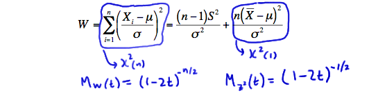
Now for proving number 2. This is one of those proofs that you might have to read through twice... perhaps reading it the first time just to see where we're going with it, and then, if necessary, reading it again to capture the details. We're going to start with a function which we'll call \(W\):
\(W=\sum\limits_{i=1}^n \left(\dfrac{X_i-\mu}{\sigma}\right)^2\)
Now, we can take \(W\) and do the trick of adding 0 to each term in the summation. Doing so, of course, doesn't change the value of \(W\):
\(W=\sum\limits_{i=1}^n \left(\dfrac{(X_i-\bar{X})+(\bar{X}-\mu)}{\sigma}\right)^2\)
As you can see, we added 0 by adding and subtracting the sample mean to the quantity in the numerator. Now, let's square the term. Doing just that, and distributing the summation, we get:
\(W=\sum\limits_{i=1}^n \left(\dfrac{X_i-\bar{X}}{\sigma}\right)^2+\sum\limits_{i=1}^n \left(\dfrac{\bar{X}-\mu}{\sigma}\right)^2+2\left(\dfrac{\bar{X}-\mu}{\sigma^2}\right)\sum\limits_{i=1}^n (X_i-\bar{X})\)
But the last term is 0:
\(W=\sum\limits_{i=1}^n \left(\dfrac{X_i-\bar{X}}{\sigma}\right)^2+\sum\limits_{i=1}^n \left(\dfrac{\bar{X}-\mu}{\sigma}\right)^2+ \underbrace{ 2\left(\dfrac{\bar{X}-\mu}{\sigma^2}\right)\sum\limits_{i=1}^n (X_i-\bar{X})}_{0, since \sum(X_i - \bar{X}) = n\bar{X}-n\bar{X}=0}\)
so, \(W\) reduces to:
\(W=\sum\limits_{i=1}^n \dfrac{(X_i-\bar{X})^2}{\sigma^2}+\dfrac{n(\bar{X}-\mu)^2}{\sigma^2}\)
We can do a bit more with the first term of \(W\). As an aside, if we take the definition of the sample variance:
\(S^2=\dfrac{1}{n-1}\sum\limits_{i=1}^n (X_i-\bar{X})^2\)
and multiply both sides by \((n-1)\), we get:
\((n-1)S^2=\sum\limits_{i=1}^n (X_i-\bar{X})^2\)
So, the numerator in the first term of \(W\) can be written as a function of the sample variance. That is:
\(W=\sum\limits_{i=1}^n \left(\dfrac{X_i-\mu}{\sigma}\right)^2=\dfrac{(n-1)S^2}{\sigma^2}+\dfrac{n(\bar{X}-\mu)^2}{\sigma^2}\)
Okay, let's take a break here to see what we have. We've taken the quantity on the left side of the above equation, added 0 to it, and showed that it equals the quantity on the right side. Now, what can we say about each of the terms. Well, the term on the left side of the equation:
\(\sum\limits_{i=1}^n \left(\dfrac{X_i-\mu}{\sigma}\right)^2\)
is a sum of \(n\) independent chi-square(1) random variables. That's because we have assumed that \(X_1, X_2, \ldots, X_n\) are observations of a random sample of size \(n\) from the normal distribution \(N(\mu, \sigma^2)\). Therefore:
\(\dfrac{X_i-\mu}{\sigma}\)
follows a standard normal distribution. Now, recall that if we square a standard normal random variable, we get a chi-square random variable with 1 degree of freedom. So, again:
\(\sum\limits_{i=1}^n \left(\dfrac{X_i-\mu}{\sigma}\right)^2\)
is a sum of \(n\) independent chi-square(1) random variables. Our work from the previous lesson then tells us that the sum is a chi-square random variable with \(n\) degrees of freedom. Therefore, the moment-generating function of \(W\) is the same as the moment-generating function of a chi-square(n) random variable, namely:
\(M_W(t)=(1-2t)^{-n/2}\)
for \(t<\frac{1}{2}\). Now, the second term of \(W\), on the right side of the equals sign, that is:
\(\dfrac{n(\bar{X}-\mu)^2}{\sigma^2}\)
is a chi-square(1) random variable. That's because the sample mean is normally distributed with mean \(\mu\) and variance \(\frac{\sigma^2}{n}\). Therefore:
\(Z=\dfrac{\bar{X}-\mu}{\sigma/\sqrt{n}}\sim N(0,1)\)
is a standard normal random variable. So, if we square \(Z\), we get a chi-square random variable with 1 degree of freedom:
\(Z^2=\dfrac{n(\bar{X}-\mu)^2}{\sigma^2}\sim \chi^2(1)\)
And therefore the moment-generating function of \(Z^2\) is:
\(M_{Z^2}(t)=(1-2t)^{-1/2}\)
for \(t<\frac{1}{2}\). Let's summarize again what we know so far. \(W\) is a chi-square(n) random variable, and the second term on the right is a chi-square(1) random variable:
Now, let's use the uniqueness property of moment-generating functions. By definition, the moment-generating function of \(W\) is:
\(M_W(t)=E(e^{tW})=E\left[e^{t((n-1)S^2/\sigma^2+Z^2)}\right]\)
Using what we know about exponents, we can rewrite the term in the expectation as a product of two exponent terms:
\(E(e^{tW})=E\left[e^{t((n-1)S^2/\sigma^2)}\cdot e^{tZ^2}\right]=M_{(n-1)S^2/\sigma^2}(t) \cdot M_{Z^2}(t)\)
The last equality in the above equation comes from the independence between \(\bar{X}\) and \(S^2\). That is, if they are independent, then functions of them are independent. Now, let's substitute in what we know about the moment-generating function of \(W\) and of \(Z^2\). Doing so, we get:
\((1-2t)^{-n/2}=M_{(n-1)S^2/\sigma^2}(t) \cdot (1-2t)^{-1/2}\)
Now, let's solve for the moment-generating function of \(\frac{(n-1)S^2}{\sigma^2}\), whose distribution we are trying to determine. Doing so, we get:
\(M_{(n-1)S^2/\sigma^2}(t)=(1-2t)^{-n/2}\cdot (1-2t)^{1/2}\)
Adding the exponents, we get:
\(M_{(n-1)S^2/\sigma^2}(t)=(1-2t)^{-(n-1)/2}\)
for \(t<\frac{1}{2}\). But, oh, that's the moment-generating function of a chi-square random variable with \(n-1\) degrees of freedom. Therefore, the uniqueness property of moment-generating functions tells us that \(\frac{(n-1)S^2}{\sigma^2}\) must be a a chi-square random variable with \(n-1\) degrees of freedom. That is:
\(\dfrac{(n-1)S^2}{\sigma^2}=\dfrac{\sum\limits_{i=1}^n (X_i-\bar{X})^2}{\sigma^2} \sim \chi^2_{(n-1)}\)
as was to be proved! And, to just think that this was the easier of the two proofs
Before we take a look at an example involving simulation, it is worth noting that in the last proof, we proved that, when sampling from a normal distribution:
\(\dfrac{\sum\limits_{i=1}^n (X_i-\mu)^2}{\sigma^2} \sim \chi^2(n)\)
but:
\(\dfrac{\sum\limits_{i=1}^n (X_i-\bar{X})^2}{\sigma^2}=\dfrac{(n-1)S^2}{\sigma^2}\sim \chi^2(n-1)\)
The only difference between these two summations is that in the first case, we are summing the squared differences from the population mean \(\mu\), while in the second case, we are summing the squared differences from the sample mean \(\bar{X}\). What happens is that when we estimate the unknown population mean \(\mu\) with\(\bar{X}\) we "lose" one degreee of freedom. This is generally true... a degree of freedom is lost for each parameter estimated in certain chi-square random variables.
Example 26-5
Let's return to our example concerning the IQs of randomly selected individuals. Let \(X_i\) denote the Stanford-Binet Intelligence Quotient (IQ) of a randomly selected individual, \(i=1, \ldots, 8\). Recalling that IQs are normally distributed with mean \(\mu=100\) and variance \(\sigma^2=16^2\), what is the distribution of \(\dfrac{(n-1)S^2}{\sigma^2}\)?
Solution
Because the sample size is \(n=8\), the above theorem tells us that:
\(\dfrac{(8-1)S^2}{\sigma^2}=\dfrac{7S^2}{\sigma^2}=\dfrac{\sum\limits_{i=1}^8 (X_i-\bar{X})^2}{\sigma^2}\)
follows a chi-square distribution with 7 degrees of freedom. Here's what the theoretical density function would look like:
Again, all the work that we have done so far concerning this example has been theoretical in nature. That is, what we have learned is based on probability theory. Would we see the same kind of result if we were take to a large number of samples, say 1000, of size 8, and calculate:
\(\dfrac{\sum\limits_{i=1}^8 (X_i-\bar{X})^2}{256}\)
for each sample? That is, would the distribution of the 1000 resulting values of the above function look like a chi-square(7) distribution? Again, the only way to answer this question is to try it out! I did just that for us. I used Minitab to generate 1000 samples of eight random numbers from a normal distribution with mean 100 and variance 256. Here's a subset of the resulting random numbers:
As you can see, the last column, titled FnofSsq (for function of sums of squares), contains the calculated value of:
\(\dfrac{\sum\limits_{i=1}^8 (X_i-\bar{X})^2}{256}\)
based on the random numbers generated in columns X1 X2, X3, X4, X5, X6, X7, and X8. For example, given that the average of the eight numbers in the first row is 98.625, the value of FnofSsq in the first row is:
\(\dfrac{1}{256}[(98-98.625)^2+(77-98.625)^2+\cdots+(91-98.625)^2]=5.7651\)
Now, all we have to do is create a histogram of the values appearing in the FnofSsq column. Doing so, we get:
Hmm! The histogram sure looks eerily similar to that of the density curve of a chi-square random variable with 7 degrees of freedom. It looks like the practice is meshing with the theory!
26.4 - Student's t Distribution
26.4 - Student's t DistributionWe have just one more topic to tackle in this lesson, namely, Student's t distribution. Let's just jump right in and define it!
Definition. If \(Z\sim N(0,1)\) and \(U\sim \chi^2(r)\) are independent, then the random variable:
\(T=\dfrac{Z}{\sqrt{U/r}}\)
follows a \(t\)-distribution with \(r\) degrees of freedom. We write \(T\sim t(r)\). The p.d.f. of T is:
\(f(t)=\dfrac{\Gamma((r+1)/2)}{\sqrt{\pi r} \Gamma(r/2)} \cdot \dfrac{1}{(1+t^2/r)^{(r+1)/2}}\)
for \(-\infty<t<\infty\).
By the way, the \(t\) distribution was first discovered by a man named W.S. Gosset. He discovered the distribution when working for an Irish brewery. Because he published under the pseudonym Student, the \(t\) distribution is often called Student's \(t\) distribution.
History aside, the above definition is probably not particularly enlightening. Let's try to get a feel for the \(t\) distribution by way of simulation. Let's randomly generate 1000 standard normal values (\(Z\)) and 1000 chi-square(3) values (\(U\)). Then, the above definition tells us that, if we take those randomly generated values, calculate:
\(T=\dfrac{Z}{\sqrt{U/3}}\)
and create a histogram of the 1000 resulting \(T\) values, we should get a histogram that looks like a \(t\) distribution with 3 degrees of freedom. Well, here's a subset of the resulting values from one such simulation:
| ROW | Z | CHISQ (3) | T(3) |
|---|---|---|---|
| 1 | -2.60481 | 10.2497 | -1.4092 |
| 2 | 2.92321 | 1.6517 | 3.9396 |
| 3 | -0.48633 | 0.1757 | -2.0099 |
| 4 | -0.48212 | 3.8283 | -0.4268 |
| 5 | -0.04150 | 0.2422 | -0.1461 |
| 6 | -0.84225 | -0.0903 | -4.8544 |
| 7 | -0.31205 | 1.6326 | -0.4230 |
| 8 | 1.33068 | 5.2224 | 1.0086 |
| 9 | -0.64104 | 0.9401 | -1.1451 |
| 10 | -0.05110 | 2.2632 | -0.0588 |
| 11 | 1.61601 | 4.6566 | 1.2971 |
| 12 | 0.81522 | 2.1738 | 0.9577 |
| 13 | 0.38501 | 1.8404 | 0.4916 |
| 14 | -1.63426 | 1.1265 | -2.6669 |
| ...and so on... | |||
| 994 | -0.18942 | 3.5202 | -0.1749 |
| 995 | 0.43078 | 3.3585 | 0.4071 |
| 996 | -0.14068 | 0.6236 | -0.3085 |
| 997 | -1.76357 | 2.6188 | -1.8876 |
| 998 | -1.02310 | 3.2470 | -0.9843 |
| 999 | -0.93777 | 1.4991 | -1.3266 |
| 1000 | -0.37665 | 2.1231 | -0.4477 |
Note, for example, in the first row:
\(T(3)=\dfrac{-2.60481}{\sqrt{10.2497/3}}=-1.4092\)
Here's what the resulting histogram of the 1000 randomly generated \(T(3)\) values looks like, with a standard \(N(0,1)\) curve superimposed:
Hmmm. The \(t\)-distribution seems to be quite similar to the standard normal distribution. Using the formula given above for the p.d.f. of \(T\), we can plot the density curve of various \(t\) random variables, say when \(r=1, r=4\), and \(r=7\), to see that that is indeed the case:
In fact, it looks as if, as the degrees of freedom \(r\) increases, the \(t\) density curve gets closer and closer to the standard normal curve. Let's summarize what we've learned in our little investigation about the characteristics of the t distribution:
- The support appears to be \(-\infty<t<\infty\). (It is!)
- The probability distribution appears to be symmetric about \(t=0\). (It is!)
- The probability distribution appears to be bell-shaped. (It is!)
- The density curve looks like a standard normal curve, but the tails of the \(t\)-distribution are "heavier" than the tails of the normal distribution. That is, we are more likely to get extreme \(t\)-values than extreme \(z\)-values.
- As the degrees of freedom \(r\) increases, the \(t\)-distribution appears to approach the standard normal \(z\)-distribution. (It does!)
As you'll soon see, we'll need to look up \(t\)-values, as well as probabilities concerning \(T\) random variables, quite often in Stat 415. Therefore, we better make sure we know how to read a \(t\) table.
The \(t\) Table
If you take a look at Table VI in the back of your textbook, you'll find what looks like a typical \(t\) table. Here's what the top of Table VI looks like (well, minus the shading that I've added):
\[P(T \leq t)=\int_{-\infty}^{t} \frac{\Gamma[(r+1) / 2]}{\sqrt{\pi r} \Gamma(r / 2)\left(1+w^{2} / r\right)^{(r+1) / 2}} d w\]
\[P(T \leq-t)=1-P(T \leq t)\]
| P(T≤ t) | |||||||
| 0.60 | 0.75 | 0.90 | 0.95 | 0.975 | 0.99 | 0.995 | |
| r | t0.40(r) | t0.25(r) | t0.10(r) | t0.05(r) | t0.025(r) | t0.01(r) | t0.005(r) |
| 1 | 0.325 | 1.000 | 3.078 | 6.314 | 12.706 | 31.821 | 63.657 |
| 2 | 0.289 | 0.816 | 1.886 | 2.920 | 4.303 | 6.965 | 9.925 |
| 3 | 0.277 | 0.765 | 1.638 | 2.353 | 3.182 | 4.541 | 5.841 |
| 4 | 0.271 | 0.741 | 1.533 | 2.132 | 2.776 | 3.747 | 4.604 |
| 5 | 0.267 | 0.727 | 1.476 | 2.015 | 2.571 | 3.365 | 4.032 |
| 6 | 0.265 | 0.718 | 1.440 | 1.943 | 2.447 | 3.143 | 3.707 |
| 7 | 0.263 | 0.711 | 1.415 | 1.895 | 2.365 | 2.998 | 3.499 |
| 8 | 0.262 | 0.706 | 1.397 | 1.860 | 2.306 | 2.896 | 3.355 |
| 9 | 0.261 | 0.703 | 1.383 | 1.833 | 2.262 | 2.821 | 3.250 |
| 10 | 0.260 | 0.700 | 1.372 | 1.812 | 2.228 | 2.764 | 3.169 |
The \(t\)-table is similar to the chi-square table in that the inside of the \(t\)-table (shaded in purple) contains the \(t\)-values for various cumulative probabilities (shaded in red), such as 0.60, 0.75, 0.90, 0.95, 0.975, 0.99, and 0.995, and for various \(t\) distributions with \(r\) degrees of freedom (shaded in blue). The row shaded in green indicates the upper \(\alpha\) probability that corresponds to the \(1-\alpha\) cumulative probability. For example, if you're interested in either a cumulative probability of 0.60, or an upper probability of 0.40, you'll want to look for the \(t\)-value in the first column.
Let's use the \(t\)-table to read a few probabilities and \(t\)-values off of the table:
Let's take a look at a few more examples.
Example 26-6
Let \(T\) follow a \(t\)-distribution with \(r=8\) df. What is the probability that the absolute value of \(T\) is less than 2.306?
Solution
The probability calculation is quite similar to a calculation we'd have to make for a normal random variable. First, rewriting the probability in terms of \(T\) instead of the absolute value of \(T\), we get:
\(P(|T|<2.306)=P(-2.306<T<2.306)\)
Then, we have to rewrite the probability in terms of cumulative probabilities that we can actually find, that is:
\(P(|T|<2.306)=P(T<2.306)-P(T<-2.306)\)
Pictorially, the probability we are looking for looks something like this:
But the \(t\)-table doesn't contain negative \(t\)-values, so we'll have to take advantage of the symmetry of the \(T\) distribution. That is:
>\(P(|T|<2.306)=P(T<2.306)-P(T>2.306)\)
| P(T≤ t) | |||||||
| 0.60 | 0.75 | 0.90 | 0.95 | 0.975 | 0.99 | 0.995 | |
| r | t0.40(r) | t0.25(r) | t0.10(r) | t0.05(r) | t0.025(r) | t0.01(r) | t0.005(r) |
| 1 | 0.325 | 1.000 | 3.078 | 6.314 | 12.706 | 31.821 | 63.657 |
| 2 | 0.289 | 0.816 | 1.886 | 2.920 | 4.303 | 6.965 | 9.925 |
| 3 | 0.277 | 0.765 | 1.638 | 2.353 | 3.182 | 4.541 | 5.841 |
| 4 | 0.271 | 0.741 | 1.533 | 2.132 | 2.776 | 3.747 | 4.604 |
| 5 | 0.267 | 0.727 | 1.476 | 2.015 | 2.571 | 3.365 | 4.032 |
| 6 | 0.265 | 0.718 | 1.440 | 1.943 | 2.447 | 3.143 | 3.707 |
| 7 | 0.263 | 0.711 | 1.415 | 1.895 | 2.365 | 2.998 | 3.499 |
| 8 | 0.262 | 0.706 | 1.397 | 1.860 | 2.306 | 2.896 | 3.355 |
| 9 | 0.261 | 0.703 | 1.383 | 1.833 | 2.262 | 2.821 | 3.250 |
| 10 | 0.260 | 0.700 | 1.372 | 1.812 | 2.228 | 2.764 | 3.169 |
The \(t\)-table tells us that \(P(T<2.306)=0.975\) and \(P(T>2.306)=0.025\). Therefore:
\(P(|T|>2.306)=0.975-0.025=0.95\)
What is \(t_{0.05}(8)\)?
Solution
The value \(t_{0.05}(8)\) is the value \(t_{0.05}\) such that the probability that a \(T\) random variable with 8 degrees of freedom is greater than the value \(t_{0.05}\) is 0.05. That is:
Can you find the value \(t_{0.05}\) on the \(t\)-table?
| P(T≤ t) | |||||||
| 0.60 | 0.75 | 0.90 | 0.95 | 0.975 | 0.99 | 0.995 | |
| r | t0.40(r) | t0.25(r) | t0.10(r) | t0.05(r) | t0.025(r) | t0.01(r) | t0.005(r) |
| 1 | 0.325 | 1.000 | 3.078 | 6.314 | 12.706 | 31.821 | 63.657 |
| 2 | 0.289 | 0.816 | 1.886 | 2.920 | 4.303 | 6.965 | 9.925 |
| 3 | 0.277 | 0.765 | 1.638 | 2.353 | 3.182 | 4.541 | 5.841 |
| 4 | 0.271 | 0.741 | 1.533 | 2.132 | 2.776 | 3.747 | 4.604 |
| 5 | 0.267 | 0.727 | 1.476 | 2.015 | 2.571 | 3.365 | 4.032 |
| 6 | 0.265 | 0.718 | 1.440 | 1.943 | 2.447 | 3.143 | 3.707 |
| 7 | 0.263 | 0.711 | 1.415 | 1.895 | 2.365 | 2.998 | 3.499 |
| 8 | 0.262 | 0.706 | 1.397 | 1.860 | 2.306 | 2.896 | 3.355 |
| 9 | 0.261 | 0.703 | 1.383 | 1.833 | 2.262 | 2.821 | 3.250 |
| 10 | 0.260 | 0.700 | 1.372 | 1.812 | 2.228 | 2.764 | 3.169 |
We have determined that the probability that a \(T\) random variable with 8 degrees of freedom is greater than the value 1.860 is 0.05.
Why will we encounter a \(T\) random variable?
Given a random sample \(X_1, X_2, \ldots, X_n\) from a normal distribution, we know that:
\(Z=\dfrac{\bar{X}-\mu}{\sigma/\sqrt{n}}\sim N(0,1)\)
Earlier in this lesson, we learned that:
\(U=\dfrac{(n-1)S^2}{\sigma^2}\)
follows a chi-square distribution with \(n-1\) degrees of freedom. We also learned that \(Z\) and \(U\) are independent. Therefore, using the definition of a \(T\) random variable, we get:
It is the resulting quantity, that is:
\(T=\dfrac{\bar{X}-\mu}{s/\sqrt{n}}\)
that will help us, in Stat 415, to use a mean from a random sample, that is \(\bar{X}\), to learn, with confidence, something about the population mean \(\mu\).