Lesson 27: The Central Limit Theorem

Introduction

In the previous lesson, we investigated the probability distribution ("sampling distribution") of the sample mean when the random sample \(X_1, X_2, \ldots, X_n\) comes from a normal population with mean \(\mu\) and variance \(\sigma^2\), that is, when \(X_i\sim N(\mu, \sigma^2), i=1, 2, \ldots, n\). Specifically, we learned that if \(X_i\), \(i=1, 2, \ldots, n\), is a random sample of size \(n\) from a \(N(\mu, \sigma^2)\) population, then:

\(\bar{X}\sim N\left(\mu,\dfrac{\sigma^2}{n}\right)\)

But what happens if the \(X_i\) follow some other non-normal distribution? For example, what distribution does the sample mean follow if the \(X_i\) come from the Uniform(0, 1) distribution? Or, what distribution does the sample mean follow if the \(X_i\) come from a chi-square distribution with three degrees of freedom? Those are the kinds of questions we'll investigate in this lesson. As the title of this lesson suggests, it is the Central Limit Theorem that will give us the answer.

Objectives

Upon completion of this lesson, you should be able to:

To learn the Central Limit Theorem.
To get an intuitive feeling for the Central Limit Theorem.
To use the Central Limit Theorem to find probabilities concerning the sample mean.
To be able to apply the methods learned in this lesson to new problems.

27.1 - The Theorem

Central Limit Theorem

We don't have the tools yet to prove the Central Limit Theorem, so we'll just go ahead and state it without proof.

Let \(X_1, X_2, \ldots, X_n\) be a random sample from a distribution (any distribution!) with (finite) mean \(\mu\) and (finite) variance \(\sigma^2\). If the sample size \(n\) is "sufficiently large," then:

the sample mean \(\bar{X}\) follows an approximate normal distribution
with mean \(E(\bar{X})=\mu_{\bar{X}}=\mu\)
and variance \(Var(\bar{X})=\sigma^2_{\bar{X}}=\dfrac{\sigma^2}{n}\)

We write:

\(\bar{X} \stackrel{d}{\longrightarrow} N\left(\mu,\dfrac{\sigma^2}{n}\right)\) as \(n\rightarrow \infty\)

or:

\(Z=\dfrac{\bar{X}-\mu}{\sigma/\sqrt{n}}=\dfrac{\sum\limits_{i=1}^n X_i-n\mu}{\sqrt{n}\sigma} \stackrel {d}{\longrightarrow} N(0,1)\) as \(n\rightarrow \infty\).

So, in a nutshell, the Central Limit Theorem (CLT) tells us that the sampling distribution of the sample mean is, at least approximately, normally distributed, regardless of the distribution of the underlying random sample. In fact, the CLT applies regardless of whether the distribution of the \(X_i\) is discrete (for example, Poisson or binomial) or continuous (for example, exponential or chi-square). Our focus in this lesson will be on continuous random variables. In the next lesson, we'll apply the CLT to discrete random variables, such as the binomial and Poisson random variables.

You might be wondering why "sufficiently large" appears in quotes in the theorem. Well, that's because the necessary sample size \(n\) depends on the skewness of the distribution from which the random sample \(X_i\) comes:

If the distribution of the \(X_i\) is symmetric, unimodal or continuous, then a sample size \(n\) as small as 4 or 5 yields an adequate approximation.
If the distribution of the \(X_i\) is skewed, then a sample size \(n\) of at least 25 or 30 yields an adequate approximation.
If the distribution of the \(X_i\) is extremely skewed, then you may need an even larger \(n\).

We'll spend the rest of the lesson trying to get an intuitive feel for the theorem, as well as applying the theorem so that we can calculate probabilities concerning the sample mean.

27.2 - Implications in Practice

As stated on the previous page, we don't yet have the tools to prove the Central Limit Theorem. And, we won't actually get to proving it until late in Stat 415. It would be good though to get an intuitive feel now for how the CLT works in practice. On this page, we'll explore two examples to get a feel for how:

the skewness (or symmetry!) of the underlying distribution of \(X_i\), and
the sample size \(n\)

affect how well the normal distribution approximates the actual ("exact") distribution of the sample mean \(\bar{X}\). Well, that's not quite true. We won't actually find the exact distribution of the sample mean in the two examples. We'll instead use simulation to do the work for us. In the first example, we'll take a look at sample means drawn from a symmetric distribution, specifically, the Uniform(0,1) distribution. In the second example, we'll take a look at sample means drawn from a highly skewed distribution, specifically, the chi-square(3) distribution. In each case, we'll see how large the sample size \(n\) has to get before the normal distribution does a decent job of approximating the simulated distribution.

Example 27-1

Consider taking random samples of various sizes \(n\) from the (symmetric) Uniform (0, 1) distribution. At what sample size \(n\) does the normal distribution make a good approximation to the actual distribution of the sample mean?

Solution

Our previous work on the continuous Uniform(0, 1) random variable tells us that the mean of a \(U(0,1)\) random variable is:

\(\mu=E(X_i)=\dfrac{0+1}{2}=\dfrac{1}{2}\)

while the variance of a \(U(0,1)\) random variable is:

\(\sigma^2=Var(X_i)=\dfrac{(1-0)^2}{12}=\dfrac{1}{12}\)

The Central Limit Theorem, therefore, tells us that the sample mean \(\bar{X}\) is approximately normally distributed with mean:

\(\mu_{\bar{X}}=\mu=\dfrac{1}{2}\)

and variance:

\(\sigma^2_{\bar{X}}=\dfrac{\sigma^2}{n}=\dfrac{1/12}{n}=\dfrac{1}{12n}\)

Now, our end goal is to compare the normal distribution, as defined by the CLT, to the actual distribution of the sample mean. Now, we could do a lot of theoretical work to find the exact distribution of \(\bar{X}\) for various sample sizes \(n\). Instead, we'll use simulation to give us a ballpark idea of the shape of the distribution of \(\bar{X}\). Here's an outline of the general strategy that we'll follow:

Specify the sample size \(n\).
Randomly generate 1000 samples of size \(n\) from the Uniform (0,1) distribution.
Use the 1000 generated samples to calculate 1000 sample means from the Uniform (0,1) distribution.
Create a histogram of the 1000 sample means.
Compare the histogram to the normal distribution, as defined by the Central Limit Theorem, in order to see how well the Central Limit Theorem works for the given sample size \(n\).

Let's start with a sample size of \(n=1\). That is, randomly sample 1000 numbers from a Uniform (0,1) distribution, and create a histogram of the 1000 generated numbers. Of course, the histogram should look roughly flat like a Uniform(0,1) distribution. If you're willing to ignore the artifacts of sampling, you can see that our histogram is roughly flat:

Okay, now let's tackle the more interesting sample sizes. Let \(n=2\). Generating 1000 samples of size \(n=2\), calculating the 1000 sample means, and creating a histogram of the 1000 sample means, we get:

It can actually be shown that the exact distribution of the sample mean of 2 numbers drawn from the Uniform(0, 1) distribution is the triangular distribution. The histogram does look a bit triangular, doesn't it? The blue curve overlaid on the histogram is the normal distribution, as defined by the Central Limit Theorem. That is, the blue curve is the normal distribution with mean:

\(\mu_{\bar{X}}=\mu=\dfrac{1}{2}\)

and variance:

\(\sigma^2_{\bar{X}}=\dfrac{1}{12n}=\dfrac{1}{12(2)}=\dfrac{1}{24}\)

As you can see, already at \(n=2\), the normal curve wouldn't do too bad of a job of approximating the exact probabilities. Let's increase the sample size to \(n=4\). Generating 1000 samples of size \(n=4\), calculating the 1000 sample means, and creating a histogram of the 1000 sample means, we get:

The blue curve overlaid on the histogram is the normal distribution, as defined by the Central Limit Theorem. That is, the blue curve is the normal distribution with mean:

\(\mu_{\bar{X}}=\mu=\dfrac{1}{2}\)

and variance:

\(\sigma^2_{\bar{X}}=\dfrac{1}{12n}=\dfrac{1}{12(4)}=\dfrac{1}{48}\)

Again, at \(n=4\), the normal curve does a very good job of approximating the exact probabilities. In fact, it does such a good job, that we could probably stop this exercise already. But let's increase the sample size to \(n=9\). Generating 1000 samples of size \(n=9\), calculating the 1000 sample means, and creating a histogram of the 1000 sample means, we get:

The blue curve overlaid on the histogram is the normal distribution, as defined by the Central Limit Theorem. That is, the blue curve is the normal distribution with mean:

\(\mu_{\bar{X}}=\mu=\dfrac{1}{2}\)

and variance:

\(\sigma^2_{\bar{X}}=\dfrac{1}{12n}=\dfrac{1}{12(9)}=\dfrac{1}{108}\)

And not surprisingly, at \(n=9\), the normal curve does a very good job of approximating the exact probabilities. There is another interesting thing worth noting though, too. As you can see, as the sample size increases, the variance of the sample mean decreases. That's a good thing, as it doesn't seem that it should be any other way. If you think about it, if it were possible to increase the sample size \(n\) to something close to the size of the population, you would expect that the resulting sample means would not vary much, and would be close to the population mean. Of course, the trade-off here is that large sample sizes typically cost lots more money than small sample sizes.

Well, just for the heck of it, let's increase our sample size one more time to \(n=16\). Generating 1000 samples of size \(n=16\), calculating the 1000 sample means, and creating a histogram of the 1000 sample means, we get:

The blue curve overlaid on the histogram is the normal distribution with mean:

\(\mu_{\bar{X}}=\mu=\dfrac{1}{2}\)

and variance:

\(\sigma^2_{\bar{X}}=\dfrac{1}{12n}=\dfrac{1}{12(16)}=\dfrac{1}{192}\)

Again, at \(n=16\), the normal curve does a very good job of approximating the exact probabilities. Okay, uncle! That's enough of this example! Let's summarize the two take-away messages from this example:

If the underlying distribution is symmetric, then you don't need a very large sample size for the normal distribution, as defined by the Central Limit Theorem, to do a decent job of approximating the probability distribution of the sample mean.
The larger the sample size \(n\), the smaller the variance of the sample mean.

Example 27-2

Now consider taking random samples of various sizes \(n\) from the (skewed) chi-square distribution with 3 degrees of freedom. At what sample size \(n\) does the normal distribution make a good approximation to the actual distribution of the sample mean?

Solution

We are going to do exactly what we did in the previous example. The only difference is that our underlying distribution here, that is, the chi-square(3) distribution, is highly-skewed. Now, our previous work on the chi-square distribution tells us that the mean of a chi-square random variable with three degrees of freedom is:

\(\mu=E(X_i)=r=3\)

while the variance of a chi-square random variable with three degrees of freedom is:

\(\sigma^2=Var(X_i)=2r=2(3)=6\)

The Central Limit Theorem, therefore, tells us that the sample mean \(\bar{X}\) is approximately normally distributed with mean:

\(\mu_{\bar{X}}=\mu=3\)

and variance:

\(\sigma^2_{\bar{X}}=\dfrac{\sigma^2}{n}=\dfrac{6}{n}\)

Again, we'll follow a strategy similar to that in the above example, namely:

Specify the sample size \(n\).
Randomly generate 1000 samples of size \(n\) from the chi-square(3) distribution.
Use the 1000 generated samples to calculate 1000 sample means from the chi-square(3) distribution.
Create a histogram of the 1000 sample means.
Compare the histogram to the normal distribution, as defined by the Central Limit Theorem, in order to see how well the Central Limit Theorem works for the given sample size \(n\).

Again, starting with a sample size of \(n=1\), we randomly sample 1000 numbers from a chi-square(3) distribution, and create a histogram of the 1000 generated numbers. Of course, the histogram should look like a (skewed) chi-square(3) distribution, as the blue curve suggests it does:

Now, let's consider samples of size \(n=2\). Generating 1000 samples of size \(n=2\), calculating the 1000 sample means, and creating a histogram of the 1000 sample means, we get:

The blue curve overlaid on the histogram is the normal distribution, as defined by the Central Limit Theorem. That is, the blue curve is the normal distribution with mean:

\(\mu_{\bar{X}}=\mu=3\)

and variance:

\(\sigma^2_{\bar{X}}=\dfrac{\sigma^2}{n}=\dfrac{6}{2}=3\)

As you can see, at \(n=2\), the normal curve wouldn't do a very job of approximating the exact probabilities. The probability distribution of the sample mean still appears to be quite skewed. Let's increase the sample size to \(n=4\). Generating 1000 samples of size \(n=4\), calculating the 1000 sample means, and creating a histogram of the 1000 sample means, we get:

The blue curve overlaid on the histogram is the normal distribution, as defined by the Central Limit Theorem. That is, the blue curve is the normal distribution with mean:

\(\mu_{\bar{X}}=\mu=3\)

and variance:

\(\sigma^2_{\bar{X}}=\dfrac{\sigma^2}{n}=\dfrac{6}{4}=1.5\)

Although, at \(n=4\), the normal curve is doing a better job of approximating the probability distribution of the sample mean, there is still much room for improvement. Let's try \(n=9\). Generating 1000 samples of size \(n=9\), calculating the 1000 sample means, and creating a histogram of the 1000 sample means, we get:

The blue curve overlaid on the histogram is the normal distribution, as defined by the Central Limit Theorem. That is, the blue curve is the normal distribution with mean:

\(\mu_{\bar{X}}=\mu=3\)

and variance:

\(\sigma^2_{\bar{X}}=\dfrac{\sigma^2}{n}=\dfrac{6}{9}=0.667\)

We're getting closer, but let's really jump up the sample size to, say, \(n=25\). Generating 1000 samples of size \(n=25\), calculating the 1000 sample means, and creating a histogram of the 1000 sample means, we get:

The blue curve overlaid on the histogram is the normal distribution, as defined by the Central Limit Theorem. That is, the blue curve is the normal distribution with mean:

\(\mu_{\bar{X}}=\mu=3\)

and variance:

\(\sigma^2_{\bar{X}}=\dfrac{\sigma^2}{n}=\dfrac{6}{25}=0.24\)

Okay, now we're talking! There's still just a teeny tiny bit of skewness in the sampling distribution. Let's increase the sample size just one more time to, say, \(n=36\). Generating 1000 samples of size \(n=36\), calculating the 1000 sample means, and creating a histogram of the 1000 sample means, we get:

The blue curve overlaid on the histogram is the normal distribution, as defined by the Central Limit Theorem. That is, the blue curve is the normal distribution with mean:

\(\mu_{\bar{X}}=\mu=3\)

and variance:

\(\sigma^2_{\bar{X}}=\dfrac{\sigma^2}{n}=\dfrac{6}{36}=0.167\)

Okay, now, I'm perfectly happy! It appears that, at \(n=36\), the normal curve does a very good job of approximating the exact probabilities. Let's summarize the two take-away messages from this example:

Again, the larger the sample size \(n\), the smaller the variance of the sample mean. Nothing new there.
If the underlying distribution is skewed, then you need a larger sample size, typically \(n>30\), for the normal distribution, as defined by the Central Limit Theorem, to do a decent job of approximating the probability distribution of the sample mean.

27.3 - Applications in Practice

Now that we have an intuitive feel for the Central Limit Theorem, let's use it in two different examples. In the first example, we use the Central Limit Theorem to describe how the sample mean behaves, and then use that behavior to calculate a probability. In the second example, we take a look at the most common use of the CLT, namely to use the theorem to test a claim.

Example 27-3

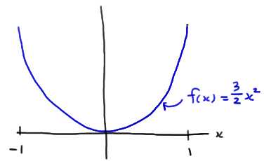
three over two all times x squared graph

Take a random sample of size \(n=15\) from a distribution whose probability density function is:

\(f(x)=\dfrac{3}{2} x^2\)

for \(-1<x<1\). What is the probability that the sample mean falls between \(-\frac{2}{5}\) and \(\frac{1}{5}\)?

Solution

The expected value of the random variable \(X\) is 0, as the following calculation illustrates:

\(\mu=E(X)=\int^1_{-1} x \cdot \dfrac{3}{2} x^2dx=\dfrac{3}{2} \int^1_{-1}x^3dx=\dfrac{3}{2} \left[\dfrac{x^4}{4}\right]^{x=1}_{x=-1}=\dfrac{3}{2} \left(\dfrac{1}{4}-\dfrac{1}{4} \right)=0\)

The variance of the random variable \(X\) is \(\frac{3}{5}\), as the following calculation illustrates:

\(\sigma^2=E(X-\mu)^2=\int^1_{-1} (x-0)^2 \dfrac{3}{2} x^2dx=\dfrac{3}{2} \int^1_{-1}x^4dx=\dfrac{3}{2} \left[\dfrac{x^5}{5}\right]^{x=1}_{x=-1}=\dfrac{3}{2} \left(\dfrac{1}{5}+\dfrac{1}{5} \right)=\dfrac{3}{5}\)

Therefore, the CLT tells us that the sample mean \(\bar{X}\) is approximately normal with mean:

\(E(\bar{X})=\mu_{\bar{X}}=\mu=0\)

and variance:

\(Var(\bar{X})=\sigma^2_{\bar{X}}=\dfrac{\sigma^2}{n}=\dfrac{3/5}{15}=\dfrac{3}{75}=\dfrac{1}{25}\)

Therefore the standard deviation of \(\bar{X}\) is \(\frac{1}{5}\). Drawing a picture of the desired probability:

we see that:

\(P(-2/5<\bar{X}<1/5)=P(-2<Z<1)\)

Therefore, using the standard normal table, we get:

\(P(-2/5<\bar{X}<1/5)=P(Z<1)-P(Z<-2)=0.8413-0.0228=0.8185\)

That is, there is an 81.85% chance that a random sample of size 15 from the given distribution will yield a sample mean between \(-\frac{2}{5}\) and \(\frac{1}{5}\).

Example 27-4

Let \(X_i\) denote the waiting time (in minutes) for the \(i^{th}\) customer. An assistant manager claims that \(\mu\), the average waiting time of the entire population of customers, is 2 minutes. The manager doesn't believe his assistant's claim, so he observes a random sample of 36 customers. The average waiting time for the 36 customers is 3.2 minutes. Should the manager reject his assistant's claim (... and fire him)?

Solution

It is reasonable to assume that \(X_i\) is an exponential random variable. And, based on the assistant manager's claim, the mean of \(X_i\) is:

\(\mu=\theta=2\).

Therefore, knowing what we know about exponential random variables, the variance of \(X_i\) is:

\(\sigma^2=\theta^2=2^2=4\).

Now, we need to know, if the mean \(\mu\) really is 2, as the assistant manager claims, what is the probability that the manager would obtain a sample mean as large as (or larger than) 3.2 minutes? Well, the Central Limit Theorem tells us that the sample mean \(\bar{X}\) is approximately normally distributed with mean:

\(\mu_{\bar{X}}=2\)

and variance:

\(\sigma^2_{\bar{X}}=\dfrac{\sigma^2}{n}=\dfrac{4}{36}=\dfrac{1}{9}\)

Here's a picture, then, of the normal probability that we need to determine:

\(z = \dfrac{3.2 - 2}{\sqrt{\frac{1}{9}}} = 3.6\)

That is:

\(P(\bar{X}>3.2)=P(Z>3.6)\)

The \(Z\) value in this case is so extreme that the table in the back of our text book can't help us find the desired probability. But, using statistical software, such as Minitab, we can determine that:

\(P(\bar{X}>3.2)=P(Z>3.6)=0.00016\)

That is, if the population mean \(\mu\) really is 2, then there is only a 16/100,000 chance (0.016%) of getting such a large sample mean. It would be quite reasonable, therefore, for the manager to reject his assistant's claim that the mean \(\mu\) is 2. The manager should feel comfortable concluding that the population mean \(\mu\) really is greater than 2. We will leave it up to him to decide whether or not he should fire his assistant!

By the way, this is the kind of example that we'll see when we study hypothesis testing in Stat 415. In general, in the process of performing a hypothesis test, someone makes a claim (the assistant, in this case), and someone collects and uses the data (the manager, in this case) to make a decision about the validity of the claim. It just so happens to be that we used the CLT in this example to help us make a decision about the assistant's claim.

^[1]	Link
↥	Has Tooltip/Popover
	Toggleable Visibility