16.6 - Some Applications
16.6 - Some ApplicationsInterpretation of Z
Note that the transformation from \(X\) to \(Z\):
\(Z=\dfrac{X-\mu}{\sigma}\)
tells us the number of standard deviations above or below the mean that \(X\) falls. That is, if \(Z=-2\), then we know that \(X\) falls 2 standard deviations below the mean. And if \(Z=+2\), then we know that \(X\) falls 2 standard deviations above the mean. As such, \(Z\)-scores are sometimes used in medical fields to identify whether an individual exhibits extreme values with respect to some biological or physical measurement.
Example 16-5
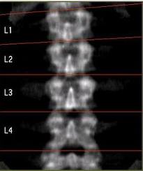
Post-menopausal women are known to be susceptible to severe bone loss known as osteoporosis. In some cases, bone loss can be so extreme as to cause a woman to lose a few inches of height. The spines and hips of women who are suspected of having osteoporosis are therefore routinely scanned to ensure that their bone loss hasn't become so severe to warrant medical intervention.
The mean \(\mu\) and standard deviation \(\sigma\) of the density of the bones in the spine, for example, are known for a healthy population. A woman is scanned and \(x\), the bone density of her spine is determined. She and her doctor would then naturally want to know whether the woman's bone density \(x\) is extreme enough to warrant medical intervention. The most common way of evaluating whether a particular \(x\) is extreme is to use the mean \(\mu\), the standard deviation \(\sigma\), and the value \(x\) to calculate a \(Z\)-score. The \(Z\)-score can then be converted to a percentile to provide the doctor and the woman an indication of the severity of her bone loss.
Suppose the woman's \(Z\)-score is −2.36, for example. The doctor then knows that the woman's bone density falls 2.36 standard deviations below the average bone density of a healthy population. The doctor, furthermore, knows that fewer than 1% of the population have a bone density more extreme than that of his/her patient.
The Empirical Rule Revisited
You might recall earlier in this section, when we investigated exploring continuous data, that we learned about the Empirical Rule. Specifically, we learned that if a histogram is at least approximately bell-shaped, then:
- approximately 68% of the data fall within one standard deviation of the mean
- approximately 95% of the data fall within two standard deviations of the mean
- approximately 99.7% of the data fall within three standard deviations of the mean
Where did those numbers come from? Now, that we've got the normal distribution under our belt, we can see why the Empirical Rule holds true. The probability that a randomly selected data value from a normal distribution falls within one standard deviation of the mean is
\(P(-1<Z<1)=P(Z<1)-P(Z>1)=0.8413-0.1587=0.6826\)
That is, we should expect 68.26% (approximately 68%!) of the data values arising from a normal population to be within one standard deviation of the mean, that is, to fall in the interval:
\((\mu-\sigma, \mu+\sigma)\)
The probability that a randomly selected data value from a normal distribution falls within two standard deviations of the mean is
\(P(-2<Z<2)=P(Z<2)-P(Z>2)=0.9772-0.0228=0.9544\)
That is, we should expect 95.44% (approximately 95%!) of the data values arising from a normal population to be within two standard deviations of the mean, that is, to fall in the interval:
\((\mu-2\sigma, \mu+2\sigma)\)
And, the probability that a randomly selected data value from a normal distribution falls within three standard deviations of the mean is:
\(P(-3<Z<3)=P(Z<3)-P(Z>3)=0.9987-0.0013=0.9974\)
That is, we should expect 99.74% (almost all!) of the data values arising from a normal population to be within three standard deviations of the mean, that is, to fall in the interval:
\((\mu-3\sigma, \mu+3\sigma)\)
Let's take a look at an example of the Empirical Rule in action.
Example 16-6
The left arm length, in inches, of 213 students were measured. Here's the resulting data, and a picture of a dot plot of the resulting arm lengths:
As you can see, the plot suggests that the distribution of the data is at least bell-shaped enough to warrant the assumption that \(X\), the left arm lengths of students, is normally distributed. We can use the raw data to determine that the average arm length of the 213 students measured is 25.167 inches, while the standard deviation is 2.095 inches. We'll then use 25.167 as an estimate of \(\mu\), the average left arm length of all college students, and 2.095 as an estimate of \(\sigma\), the standard deviation of the left arm lengths of all college students.
The Empirical Rule tells us then that we should expect approximately 68% of all college students to have a left arm length between:
\(\bar{x}-s=25.167-2.095=23.072\) and \(\bar{x}+s=25.167+2.095=27.262\)
inches. We should also expect approximately 95% of all college students to have a left arm length between:
\(\bar{x}-2s=25.167-2(2.095)=20.977\) and \(\bar{x}+2s=25.167+2(2.095)=29.357\)
inches. And, we should also expect approximately 99.7% of all college students to have a left arm length between:
\(\bar{x}-3s=25.167-3(2.095)=18.882\) and \(\bar{x}+3s=25.167+3(2.095)=31.452\)
Let's see what percentage of our 213 arm lengths fall in each of these intervals! It takes some work if you try to do it by hand, but statistical software can quickly determine that:
- 143, or 67.14%, of the 213 arm lengths fall in the first interval
- 204, or 95.77%, of the 213 arm lengths fall in the second interval
- 213, or 100%, of the 213 arm lengths fall in the third interval
The Empirical Rule didn't do too badly, eh?