26.3 - Sampling Distribution of Sample Variance
26.3 - Sampling Distribution of Sample VarianceNow that we've got the sampling distribution of the sample mean down, let's turn our attention to finding the sampling distribution of the sample variance. The following theorem will do the trick for us!
- \(X_1, X_2, \ldots, X_n\) are observations of a random sample of size \(n\) from the normal distribution \(N(\mu, \sigma^2)\)
- \(\bar{X}=\dfrac{1}{n}\sum\limits_{i=1}^n X_i\) is the sample mean of the \(n\) observations, and
- \(S^2=\dfrac{1}{n-1}\sum\limits_{i=1}^n (X_i-\bar{X})^2\) is the sample variance of the \(n\) observations.
Then:
- \(\bar{X}\)and \(S^2\) are independent
- \(\dfrac{(n-1)S^2}{\sigma^2}=\dfrac{\sum_{i=1}^n (X_i-\bar{X})^2}{\sigma^2}\sim \chi^2(n-1)\)
Proof
The proof of number 1 is quite easy. Errr, actually not! It is quite easy in this course, because it is beyond the scope of the course. So, we'll just have to state it without proof.
Now for proving number 2. This is one of those proofs that you might have to read through twice... perhaps reading it the first time just to see where we're going with it, and then, if necessary, reading it again to capture the details. We're going to start with a function which we'll call \(W\):
\(W=\sum\limits_{i=1}^n \left(\dfrac{X_i-\mu}{\sigma}\right)^2\)
Now, we can take \(W\) and do the trick of adding 0 to each term in the summation. Doing so, of course, doesn't change the value of \(W\):
\(W=\sum\limits_{i=1}^n \left(\dfrac{(X_i-\bar{X})+(\bar{X}-\mu)}{\sigma}\right)^2\)
As you can see, we added 0 by adding and subtracting the sample mean to the quantity in the numerator. Now, let's square the term. Doing just that, and distributing the summation, we get:
\(W=\sum\limits_{i=1}^n \left(\dfrac{X_i-\bar{X}}{\sigma}\right)^2+\sum\limits_{i=1}^n \left(\dfrac{\bar{X}-\mu}{\sigma}\right)^2+2\left(\dfrac{\bar{X}-\mu}{\sigma^2}\right)\sum\limits_{i=1}^n (X_i-\bar{X})\)
But the last term is 0:
\(W=\sum\limits_{i=1}^n \left(\dfrac{X_i-\bar{X}}{\sigma}\right)^2+\sum\limits_{i=1}^n \left(\dfrac{\bar{X}-\mu}{\sigma}\right)^2+ \underbrace{ 2\left(\dfrac{\bar{X}-\mu}{\sigma^2}\right)\sum\limits_{i=1}^n (X_i-\bar{X})}_{0, since \sum(X_i - \bar{X}) = n\bar{X}-n\bar{X}=0}\)
so, \(W\) reduces to:
\(W=\sum\limits_{i=1}^n \dfrac{(X_i-\bar{X})^2}{\sigma^2}+\dfrac{n(\bar{X}-\mu)^2}{\sigma^2}\)
We can do a bit more with the first term of \(W\). As an aside, if we take the definition of the sample variance:
\(S^2=\dfrac{1}{n-1}\sum\limits_{i=1}^n (X_i-\bar{X})^2\)
and multiply both sides by \((n-1)\), we get:
\((n-1)S^2=\sum\limits_{i=1}^n (X_i-\bar{X})^2\)
So, the numerator in the first term of \(W\) can be written as a function of the sample variance. That is:
\(W=\sum\limits_{i=1}^n \left(\dfrac{X_i-\mu}{\sigma}\right)^2=\dfrac{(n-1)S^2}{\sigma^2}+\dfrac{n(\bar{X}-\mu)^2}{\sigma^2}\)
Okay, let's take a break here to see what we have. We've taken the quantity on the left side of the above equation, added 0 to it, and showed that it equals the quantity on the right side. Now, what can we say about each of the terms. Well, the term on the left side of the equation:
\(\sum\limits_{i=1}^n \left(\dfrac{X_i-\mu}{\sigma}\right)^2\)
is a sum of \(n\) independent chi-square(1) random variables. That's because we have assumed that \(X_1, X_2, \ldots, X_n\) are observations of a random sample of size \(n\) from the normal distribution \(N(\mu, \sigma^2)\). Therefore:
\(\dfrac{X_i-\mu}{\sigma}\)
follows a standard normal distribution. Now, recall that if we square a standard normal random variable, we get a chi-square random variable with 1 degree of freedom. So, again:
\(\sum\limits_{i=1}^n \left(\dfrac{X_i-\mu}{\sigma}\right)^2\)
is a sum of \(n\) independent chi-square(1) random variables. Our work from the previous lesson then tells us that the sum is a chi-square random variable with \(n\) degrees of freedom. Therefore, the moment-generating function of \(W\) is the same as the moment-generating function of a chi-square(n) random variable, namely:
\(M_W(t)=(1-2t)^{-n/2}\)
for \(t<\frac{1}{2}\). Now, the second term of \(W\), on the right side of the equals sign, that is:
\(\dfrac{n(\bar{X}-\mu)^2}{\sigma^2}\)
is a chi-square(1) random variable. That's because the sample mean is normally distributed with mean \(\mu\) and variance \(\frac{\sigma^2}{n}\). Therefore:
\(Z=\dfrac{\bar{X}-\mu}{\sigma/\sqrt{n}}\sim N(0,1)\)
is a standard normal random variable. So, if we square \(Z\), we get a chi-square random variable with 1 degree of freedom:
\(Z^2=\dfrac{n(\bar{X}-\mu)^2}{\sigma^2}\sim \chi^2(1)\)
And therefore the moment-generating function of \(Z^2\) is:
\(M_{Z^2}(t)=(1-2t)^{-1/2}\)
for \(t<\frac{1}{2}\). Let's summarize again what we know so far. \(W\) is a chi-square(n) random variable, and the second term on the right is a chi-square(1) random variable:
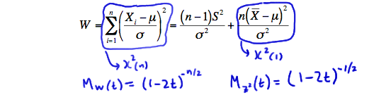
Now, let's use the uniqueness property of moment-generating functions. By definition, the moment-generating function of \(W\) is:
\(M_W(t)=E(e^{tW})=E\left[e^{t((n-1)S^2/\sigma^2+Z^2)}\right]\)
Using what we know about exponents, we can rewrite the term in the expectation as a product of two exponent terms:
\(E(e^{tW})=E\left[e^{t((n-1)S^2/\sigma^2)}\cdot e^{tZ^2}\right]=M_{(n-1)S^2/\sigma^2}(t) \cdot M_{Z^2}(t)\)
The last equality in the above equation comes from the independence between \(\bar{X}\) and \(S^2\). That is, if they are independent, then functions of them are independent. Now, let's substitute in what we know about the moment-generating function of \(W\) and of \(Z^2\). Doing so, we get:
\((1-2t)^{-n/2}=M_{(n-1)S^2/\sigma^2}(t) \cdot (1-2t)^{-1/2}\)
Now, let's solve for the moment-generating function of \(\frac{(n-1)S^2}{\sigma^2}\), whose distribution we are trying to determine. Doing so, we get:
\(M_{(n-1)S^2/\sigma^2}(t)=(1-2t)^{-n/2}\cdot (1-2t)^{1/2}\)
Adding the exponents, we get:
\(M_{(n-1)S^2/\sigma^2}(t)=(1-2t)^{-(n-1)/2}\)
for \(t<\frac{1}{2}\). But, oh, that's the moment-generating function of a chi-square random variable with \(n-1\) degrees of freedom. Therefore, the uniqueness property of moment-generating functions tells us that \(\frac{(n-1)S^2}{\sigma^2}\) must be a a chi-square random variable with \(n-1\) degrees of freedom. That is:
\(\dfrac{(n-1)S^2}{\sigma^2}=\dfrac{\sum\limits_{i=1}^n (X_i-\bar{X})^2}{\sigma^2} \sim \chi^2_{(n-1)}\)
as was to be proved! And, to just think that this was the easier of the two proofs
Before we take a look at an example involving simulation, it is worth noting that in the last proof, we proved that, when sampling from a normal distribution:
\(\dfrac{\sum\limits_{i=1}^n (X_i-\mu)^2}{\sigma^2} \sim \chi^2(n)\)
but:
\(\dfrac{\sum\limits_{i=1}^n (X_i-\bar{X})^2}{\sigma^2}=\dfrac{(n-1)S^2}{\sigma^2}\sim \chi^2(n-1)\)
The only difference between these two summations is that in the first case, we are summing the squared differences from the population mean \(\mu\), while in the second case, we are summing the squared differences from the sample mean \(\bar{X}\). What happens is that when we estimate the unknown population mean \(\mu\) with\(\bar{X}\) we "lose" one degreee of freedom. This is generally true... a degree of freedom is lost for each parameter estimated in certain chi-square random variables.
Example 26-5
Let's return to our example concerning the IQs of randomly selected individuals. Let \(X_i\) denote the Stanford-Binet Intelligence Quotient (IQ) of a randomly selected individual, \(i=1, \ldots, 8\). Recalling that IQs are normally distributed with mean \(\mu=100\) and variance \(\sigma^2=16^2\), what is the distribution of \(\dfrac{(n-1)S^2}{\sigma^2}\)?
Solution
Because the sample size is \(n=8\), the above theorem tells us that:
\(\dfrac{(8-1)S^2}{\sigma^2}=\dfrac{7S^2}{\sigma^2}=\dfrac{\sum\limits_{i=1}^8 (X_i-\bar{X})^2}{\sigma^2}\)
follows a chi-square distribution with 7 degrees of freedom. Here's what the theoretical density function would look like:
Again, all the work that we have done so far concerning this example has been theoretical in nature. That is, what we have learned is based on probability theory. Would we see the same kind of result if we were take to a large number of samples, say 1000, of size 8, and calculate:
\(\dfrac{\sum\limits_{i=1}^8 (X_i-\bar{X})^2}{256}\)
for each sample? That is, would the distribution of the 1000 resulting values of the above function look like a chi-square(7) distribution? Again, the only way to answer this question is to try it out! I did just that for us. I used Minitab to generate 1000 samples of eight random numbers from a normal distribution with mean 100 and variance 256. Here's a subset of the resulting random numbers:
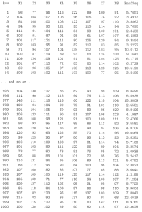
As you can see, the last column, titled FnofSsq (for function of sums of squares), contains the calculated value of:
\(\dfrac{\sum\limits_{i=1}^8 (X_i-\bar{X})^2}{256}\)
based on the random numbers generated in columns X1 X2, X3, X4, X5, X6, X7, and X8. For example, given that the average of the eight numbers in the first row is 98.625, the value of FnofSsq in the first row is:
\(\dfrac{1}{256}[(98-98.625)^2+(77-98.625)^2+\cdots+(91-98.625)^2]=5.7651\)
Now, all we have to do is create a histogram of the values appearing in the FnofSsq column. Doing so, we get:
Hmm! The histogram sure looks eerily similar to that of the density curve of a chi-square random variable with 7 degrees of freedom. It looks like the practice is meshing with the theory!