2.1 - The Situation

Point estimates, such as the sample proportion ($\hat{p}$), the sample mean ($\bar{x}$), and the sample variance ($s^2$) depend on the particular sample selected. For example:

We might know that $\hat{p}$ , the proportion of a sample of 88 students who use the city bus daily to get to campus, is 0.38. But, the bus company doesn't want to know the sample proportion. The bus company wants to know population proportion $p$, the proportion of all of the students in town who use the city bus daily.
We might know that $\bar{x}$, the average number of credit cards of 32 randomly selected American college students is 2.2. But, we want to know $\mu$, the average number of credit cards of all American college students.

The Problem

When we use the sample mean $\bar{x}$ to estimate the population mean $\mu$, can we be confident that $\bar{x}$ is close to $\mu$? And, when we use the sample proportion $\hat{p}$ to estimate the population proportion $p$, can we be confident that $\hat{p}$ is close to $p$?
Do we have any idea as to how close the sample statistic is to the population parameter?

A Solution

Rather than using just a point estimate, we could find an interval (or range) of values that we can be really confident contains the actual unknown population parameter. For example, we could find lower ($L$) and upper ($U$) values between which we can be really confident the population mean falls:

$L<\mu<U$

And, we could find lower ($L$) and upper ($U$) values between which we can be really confident the population proportion falls:

$L<p<U$

An interval of such values is called a confidence interval. Each interval has a confidence coefficient (reported as a proportion):

$1-\alpha$

or a confidence level (reported as a percentage):

$(1-\alpha)100\%$

Typical confidence coefficients are 0.90, 0.95, and 0.99, with corresponding confidence levels 90%, 95%, and 99%. For example, upon calculating a confidence interval for a mean with a confidence level of, say 95%, we can say:

"We can be 95% confident that the population mean falls between $L$ and $U$."

As should agree with our intuition, the greater the confidence level, the more confident we can be that the confidence interval contains the actual population parameter.

2.2 - A Z-Interval for a Mean

Now that we have a general idea of what a confidence interval is, we'll now turn our attention to deriving a particular confidence interval, namely that of a population mean $\mu$. We'll jump right ahead to the punch line and then back off and prove the result. But, before stating the result, we need to remind ourselves of a bit of notation.

Recall that the value:

$z_{\alpha/2}$

is the $Z$-value (obtained from a standard normal table) such that the area to the right of it under the standard normal curve is $\dfrac{\alpha}{2}$. That is:

$P(Z\geq z_{\alpha/2})=\alpha/2$

Likewise:

$-z_{\alpha/2}$

is the $Z$-value (obtained from a standard normal table) such that the area to the left of it under the standard normal curve is $\dfrac{\alpha}{2}$. That is:

$P(Z\leq -z_{\alpha/2})=\alpha/2$

I like to illustrate this notation with the following diagram of a standard normal curve:

With the notation now recalled, let's state the formula for a confidence interval for the population mean.

Theorem

$X_1, X_2, \ldots, X_n$ is a random sample from a normal population with mean $\mu$ and variance $\sigma^2$. So that:

$\bar{X}\sim N\left(\mu,\dfrac{\sigma^2}{n}\right)$ and $Z=\dfrac{\bar{X}-\mu}{\sigma/\sqrt{n}}\sim N(0,1)$
The population variance $\sigma^2$is known.

Then, a $(1-\alpha)100\%$ confidence interval for the mean $\mu$ is:

$\bar{x}\pm z_{\alpha/2}\left(\dfrac{\sigma}{\sqrt{n}}\right)$

The interval, because it depends on $Z$, is often referred to as the $Z$-interval for a mean.

Since, at this point, we're just interested in learning the basics of how to derive a confidence interval, we are going to ignore, for now, that the second assumption about the population variance being known is unrealistic. After all, when would we ever think we would know the value of the population variance $\sigma^2$, but not the population mean $\mu$? Go figure! We'll work on finding a practical confidence interval for the mean $\mu$ later. For now, let's work on deriving this one.

Proof

From the above diagram of the standard normal curve, we can see that the following probability statement is true:

$P[-z_{\alpha/2}\leq Z \leq z_{\alpha/2}]=1-\alpha $

Then, simply replacing $Z$, we get:

$P[-z_{\alpha/2}\leq \dfrac{\bar{X}-\mu}{\sigma/\sqrt{n}} \leq z_{\alpha/2}]=1-\alpha $

Now, let's focus only on manipulating the inequality inside the brackets for a bit. Because we manipulate each of the three sides of the inequality equally, each of the following statements are equivalent:

\begin{array}{rccl} -z_{\alpha/2} & \leq & \dfrac{\bar{X}-\mu}{\sigma/\sqrt{n}} & \leq & z_{\alpha/2}\\ -z_{\alpha/2}\left(\dfrac{\sigma}{\sqrt{n}}\right) & \leq & \bar{X}-\mu & \leq & +z_{\alpha/2}\left(\dfrac{\sigma}{\sqrt{n}}\right)\\ -\bar{X}-z_{\alpha/2}\left(\dfrac{\sigma}{\sqrt{n}}\right) & \leq & -\mu & \leq & -\bar{X}+z_{\alpha/2}\left(\dfrac{\sigma}{\sqrt{n}}\right)\\ \bar{X}-z_{\alpha/2}\left(\dfrac{\sigma}{\sqrt{n}}\right) & \leq & \mu &\leq & \bar{X}+z_{\alpha/2}\left(\dfrac{\sigma}{\sqrt{n}}\right) \end{array}

So, in summary, by manipulating the inequality, we have shown that the following probability statement is true:

$P\left[ \bar{X}-z_{\alpha/2}\left(\dfrac{\sigma}{\sqrt{n}}\right) \leq \mu \leq \bar{X}+z_{\alpha/2}\left(\dfrac{\sigma}{\sqrt{n}}\right) \right]=1-\alpha$

In reality, we'll learn on the next page why we shouldn't (and therefore don't!) write the formula for the $Z$-interval for the mean quite like that. Instead, we write that we can be |((1-\alpha)100\%\) confident that the mean $\mu$ is in the interval:

$\left[ \bar{x}-z_{\alpha/2}\left(\dfrac{\sigma}{\sqrt{n}}\right), \bar{x}+z_{\alpha/2}\left(\dfrac{\sigma}{\sqrt{n}}\right)\right]$

Example 2-1

A random sample of 126 police officers subjected to constant inhalation of automobile exhaust fumes in downtown Cairo had an average blood lead level concentration of 29.2 $\mu g/dl$. Assume $X$, the blood lead level of a randomly selected policeman, is normally distributed with a standard deviation of $\sigma=7.5$ $\mu g/dl$. Historically, it is known that the average blood lead level concentration of humans with no exposure to automobile exhaust is 18.2 $\mu g/dl$. Is there convincing evidence that policemen exposed to constant auto exhaust have elevated blood lead level concentrations? (Data source: Kamal, Eldamaty, and Faris, "Blood lead level of Cairo traffic policemen," Science of the Total Environment, 105(1991): 165-170.)

Answer

Let's try to answer the question by calculating a 95% confidence interval for the population mean. For a 95% confidence interval, $1-\alpha=0.95$, so that $\alpha=0.05$ and $\dfrac{\alpha}{2}=0.025$. Therefore, as the following diagram illustrates the situation, $z_{0.025}=1.96$:

Now, substituting in what we know ($\bar{x}$ = 29.2, $n=126$, $\sigma=7.5$, and $z_{0.025}=1.96$) into the the formula for a $Z$-interval for a mean, we get:

$\left[29.2-1.96\left(\dfrac{7.5}{\sqrt{126}}\right),29.2+1.96\left(\dfrac{7.5}{\sqrt{126}}\right)\right]$

Simplifying, we get a 95% confidence interval for the mean blood lead level concentration of all policemen exposed to constant auto exhaust:

$[27.89,30.51]$

That is, we can be 95% confident that the mean blood lead level concentration of all policemen exposed to constant auto exhaust is between $27.9 \mu g/dl$ and $30.5 \mu g/dl$. Note that the interval does not contain the value 18.2, the average blood lead level concentration of humans with no exposure to automobile exhaust. In fact, all of the values in the confidence interval are much greater than 18.2. Therefore, there is convincing evidence that policemen exposed to constant auto exhaust have elevated blood lead level concentrations.

Using Minitab

Statistical software, such as Minitab, can make calculating confidence intervals easier. To ask Minitab to calculate a confidence interval for a mean $\mu$, with an assumed population standard deviation, you need to do this:

Under the Stat menu, select Basic Statistics, and then select 1-Sample Z...:

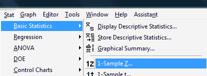
The dot-dot-dot (...) that appears after 1-Sample Z is Minitab's way of telling you that you should expect a pop-up window to appear when you click on it.
In the pop-up window that does appear, click on the radio button labeled Summarized data. Then, enter the Sample size, Mean, and Standard deviation in the boxes provided. Here's what the completed pop-up window would look like for the example above.
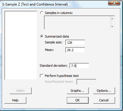
Select OK. The confidence interval output will appear in the Session window. Here is what the Minitab output would like for the example above:

One-Sample Z
The assumed standard deviation = 7.5
N Mean StDev 95% CI
126 29.2000 0.6682 (27.9804, 30.5096)

N	Mean	StDev	95% CI
126	29.2000	0.6682	(27.9804, 30.5096)

2.3 - Interpretation

The topic of interpreting confidence intervals is one that can get frequentist statisticians all hot under the collar. Let's try to understand why!

Although the derivation of the $Z$-interval for a mean technically ends with the following probability statement:

$P\left[ \bar{X}-z_{\alpha/2}\left(\dfrac{\sigma}{\sqrt{n}}\right) \leq \mu \leq \bar{X}+z_{\alpha/2}\left(\dfrac{\sigma}{\sqrt{n}}\right) \right]=1-\alpha$

it is incorrect to say:

The probability that the population mean $\mu$ falls between the lower value $L$ and the upper value $U$ is $1-\alpha$.

For example, in the example on the last page, it is incorrect to say that "the probability that the population mean is between 27.9 and 30.5 is 0.95."

Try it!

Why is it incorrect to say: "The probability that the population mean falls between the lower value $L$ and the upper value $U$ is $1-\alpha$"?

Probability statements are about random variables. The population mean $\mu$ is a constant, not a random variable. It makes no sense to make a probability statement about a constant that does not change.

So, in short, frequentist statisticians don't like to hear people trying to make probability statements about constants, when they should only be making probability statements about random variables. So, okay, if it's incorrect to make the statement that seems obvious to make based on the above probability statement, what is the correct understanding of confidence intervals? Here's how frequentist statisticians would like the world to think about confidence intervals:

Suppose we take a large number of samples, say 1000.
Then, we calculate a 95% confidence interval for each sample.
Then, "95% confident" means that we'd expect 95%, or 950, of the 1000 intervals to be correct, that is, to contain the actual unknown value $\mu$.

So, what does this all mean in practice?

In reality, we take just one random sample. The interval we obtain is either correct or incorrect. That is, the interval we obtain based on the sample we've taken either contains the true population mean or it does not. Since we don't know the value of the true population mean, we'll never know for sure whether our interval is correct or not. We can just be very confident that we obtained a correct interval (because 95% of the intervals we could have obtained are correct).

2.4 - An Interval's Length

The definition of the length of a confidence interval is perhaps obvious, but let's formally define it anyway.

Length of the Interval

If a confidence interval for a parameter $\theta$ is:

$L<\theta<U$

then the length of the interval is simply the difference in the two endpoints. That is:

$\text{Length} = U − L$

We are most interested, of course, in obtaining confidence intervals that are as narrow as possible. After all, which one of the following statements is more helpful?

We can be 95% confident that the average amount of money spent monthly on housing in the U.S. is between \$300 and \$3300.
We can be 95% confident that the average amount of money spent monthly on housing in the U.S. is between \$1100 and \$1300.

In the first statement, the average amount of money spent monthly can be anywhere between \$300 and \$3300, whereas, for the second statement, the average amount has been narrowed down to somewhere between \$1100 and \$1300. So, of course, we would prefer to make the second statement, because it gives us a more specific range of the magnitude of the population mean.

So, what can we do to ensure that we obtain as narrow an interval as possible? Well, in the case of the $Z$-interval, the length is:

$Length=\left[\bar{X}+z_{\alpha/2}\left(\dfrac{\sigma}{\sqrt{n}}\right)\right]-\left[ \bar{X}-z_{\alpha/2}\left(\dfrac{\sigma}{\sqrt{n}}\right)\right]$

which upon simplification equals:

$Length=2z_{\alpha/2}\left(\dfrac{\sigma}{\sqrt{n}}\right)$

Now, based on this formula, it looks like three factors affect the length of the $Z$-interval for a mean, namely the sample size $n$, the population standard deviation $\sigma$, and the confidence level (through the value of $z$). Specifically, the formula tells us that:

As the population standard deviation $\sigma$ decreases, the length of the interval decreases. We have no control over the population standard deviation $\sigma$, so this factor doesn't help us all that much.
As the sample size $n$ increases, the length of the interval decreases. The moral of the story, then, is to select as large of a sample as you can afford.
As the confidence level decreases, the length of the interval decreases. (Consider, for example, that for a 95% interval, $z=1.96$, whereas for a 90% interval, $z=1.645$.) So, for this factor, we have a bit of a tradeoff! We want a high confidence level, but not so high as to produce such a wide interval as to be useless. That's why 95% is the most common confidence level used.

2.5 - A t-Interval for a Mean

Our work so far

So far, we have shown that the formula:

$\bar{x}\pm z_{\alpha/2}\left(\dfrac{\sigma}{\sqrt{n}}\right)$

is appropriate for finding a confidence interval for a population mean if two conditions are met:

The population standard deviation $\sigma$ is known, and
$X_1, X_2, \ldots, X_n$ are normally distributed. (The truth is that $X_1, X_2, \ldots, X_n$ need not be normally distributed as long as the sample size $n$ is large enough for the Central Limit Theorem to apply. In this case, the confidence interval is an approximate confidence interval.)

Now, as suggested earlier in this lesson, it is unrealistic to think that we'd ever be in a situation where the first condition would be met. That is, when would we ever know the population standard deviation $\sigma$, but not the population mean $\mu$? Let's entertain, then, the realistic situation in which not only the population mean $\mu$ is unknown, but also the population standard deviation $\sigma$ is unknown.

What if $\sigma$ is unknown?

Try It!

What would be a reasonable thing to do if the population standard deviation $\sigma$ is unknown?

Estimate it with the sample standard deviation, $S$!

Yes, the reasonable thing to do is to estimate the population standard deviation $\sigma$ with the sample standard deviation:

$S=\sqrt{\dfrac{1}{n-1}\sum\limits_{i=1}^n (X_i-\bar{X})^2}$

Then, in deriving the confidence interval, we'd start out with:

$\dfrac{\bar{X}-\mu}{S/\sqrt{n}}$

instead of:

$\dfrac{\bar{X}-\mu}{\sigma/\sqrt{n}}\sim N(0,1)$

Then, to derive the confidence interval, in this case, we just need to know how:

$T=\dfrac{\bar{X}-\mu}{S/\sqrt{n}}$

is distributed!

How is $T=\dfrac{\bar{X}-\mu}{S/\sqrt{n}}$ distributed?

Given that the ratio is typically denoted by the capital letter $T$, we probably shouldn't be surprised that the ratio follows a $T$ distribution!

Theorem

If $X_1, X_2, \ldots, X_n$ are normally distributed with mean $\mu$ and variance $\sigma^2$, then:

$T=\dfrac{\bar{X}-\mu}{S/\sqrt{n}}$

follows a $T$ distribution with $n-1$ degrees of freedom.

Proof

The proof is as simple as recalling a few distributional results from our work in Stat 414. Recall the definition of a $T$ random variable, namely if $Z\sim N(0,1)$ and $U\sim \chi^2_{(r)}$ are independent, then:

$T=\dfrac{Z}{\sqrt{U/r}}$

follows the $T$ distribution with $r$ degrees of freedom. Furthermore, recall that if $X_1, X_2, \ldots, X_n$ are normally distributed with mean $\mu$ and variance $\sigma^2$, then:

$Z=\dfrac{\bar{X}-\mu}{\sigma/\sqrt{n}}\sim N(0,1)$
$\dfrac{(n-1)S^2}{\sigma^2}\sim \chi^2_{n-1}$
$\bar{X}$ and $S^2$ are independent

Now, we just have to put all that we've remembered together:

$T=\dfrac{ \frac{\bar{x}-\mu}{\sigma/\sqrt{n}} }{\sqrt{\frac{\frac{(n-1)s^2}{\sigma^2}}{n-1}}}=\dfrac{\bar{x}-\mu}{\sigma/\sqrt{n}}\left(\frac{\sigma}{s}\right)=\dfrac{\bar{x}-\mu}{s/\sqrt{n}}\sim t_{n-1}$

The first equality simply defines a $T$ random variable using the first, second, and third bullet point above. The second equality comes from canceling out the $n-1$ terms in the denominator. The third equality comes from canceling out the $\sigma$ terms, leaving us with:

$T=\dfrac{\bar{X}-\mu}{S/\sqrt{n}}$

following a $T$ distribution with $n-1$ degrees of freedom, as was to be proved!

Now that we have the distribution of $T=\dfrac{\bar{X}-\mu}{S/\sqrt{n}}$ behind us, we can derive the confidence interval for a population mean in the realistic situation that $\sigma$ is unknown.

Theorem

If $X_1, X_2, \ldots, X_n$ are normally distributed random variables with mean $\mu$ and variance $\sigma^2$, then a $(1-\alpha)100\%$ confidence interval for the population mean $\mu$ is:

$\bar{x}\pm t_{\alpha/2,n-1}\left(\dfrac{s}{\sqrt{n}}\right)$

This interval is often referred to as the "$t$-interval for the mean."

Proof

The proof is very similar to that for the $Z$-interval for the mean. We start by drawing a picture of a $T$-distribution with $n-1$ degrees of freedom:

From the diagram, we can see that the following probability statement is true:

$P[-t_{\alpha/2,n-1}\leq T \leq t_{\alpha/2,n-1}]=1-\alpha $

Then, simply replacing $T$, we get:

$P\left[-t_{\alpha/2,n-1}\leq \dfrac{\bar{X}-\mu}{s/\sqrt{n}} \leq t_{\alpha/2,n-1}\right]=1-\alpha $

Let's again focus only on the inequality inside the brackets for a bit. Because we manipulate each of the three sides of the inequality equally, each of the following statements are equivalent:

\begin{array}{rccl} -t_{\alpha/2,n-1} & \leq & \dfrac{\bar{X}-\mu}{s/\sqrt{n}} & \leq & t_{\alpha/2,n-1}\\ -t_{\alpha/2,n-1}\left(\dfrac{s}{\sqrt{n}}\right) & \leq & \bar{X}-\mu & \leq & +t_{\alpha/2,n-1}\left(\dfrac{s}{\sqrt{n}}\right)\\ -\bar{X}-t_{\alpha/2,n-1}\left(\dfrac{s}{\sqrt{n}}\right) & \leq & -\mu & \leq & -\bar{X}+t_{\alpha/2,n-1}\left(\dfrac{s}{\sqrt{n}}\right)\\ \bar{X}-t_{\alpha/2,n-1}\left(\dfrac{s}{\sqrt{n}}\right) & \leq & \mu &\leq & \bar{X}+t_{\alpha/2,n-1}\left(\dfrac{s}{\sqrt{n}}\right) \end{array}

That is, we have shown that a $(1-\alpha)100\%$ confidence interval for the mean $\mu$ is:

$\left[\bar{X}-t_{\alpha/2,n-1}\left(\dfrac{s}{\sqrt{n}}\right),\bar{X}+t_{\alpha/2,n-1}\left(\dfrac{s}{\sqrt{n}}\right)\right]$

as was to be proved.

Just one more thing. Before we go off and work through an example, let's clarify a bit of confidence interval terminology.

$t$-interval

With the formula for the $t$-interval:

$\bar{x}\pm t_{\alpha/2,n-1}\left(\dfrac{s}{\sqrt{n}}\right)$

in mind, we say that:

$\bar{x}$ is a "point estimate" of $\mu$
$\bar{x}\pm t_{\alpha/2,n-1}\left(\dfrac{s}{\sqrt{n}}\right)$ is an "interval estimate" of $\mu$
$\dfrac{s}{\sqrt{n}}$ is the "standard error of the mean"
$t_{\alpha/2,n-1}\left(\dfrac{s}{\sqrt{n}}\right)$ is the "margin of error"

Now, let's take a look at an example!

Example 2-2

A random sample of 16 Americans yielded the following data on the number of pounds of beef consumed per year:

118 115 125 110 112 130 117 112 115 120 113 118 119 122 123 126

What is the average number of pounds of beef consumed each year per person in the United States?

Answer

To help answer the question, we'll calculate a 95% confidence interval for the mean. As the above theorem states, in order for the $t$-interval for the mean to be appropriate, the data must follow a normal distribution. We can use a normal probability plot to provide evidence that the data are (sufficiently) normally distributed:

That is, because the data points fall at least approximately on a straight line, there's no reason to conclude that the data are not normally distributed. That's convoluted statistician talk for "we're good to go." Now, punching the $n=16$ data points into a calculator (or statistical software), we can easily determine that the sample mean is 118.44 and the sample standard deviation is 5.66. For a 95% confidence interval with $n=16$ data points, we need:

$t_{0.025,15}=2.1314$

Now, we have all of the necessary elements to calculate the 95% confidence interval for the mean. It is:

$\bar{x}\pm t_{0.025,15}\left(\dfrac{s}{\sqrt{n}}\right)=118.44\pm 2.1314\left(\dfrac{5.66}{\sqrt{16}}\right)$

Simplifying, we get:

$118.44\pm 3.016$

or:

$(115.42,121.46)$

That is, we can 95% confident that the average amount of beef consumed each year per person in the United States is between 115.42 and 121.46 pounds. Wow, that's a lot of beef!

Minitab^®

Using Minitab

Again, statistical software, such as Minitab, can make calculating confidence intervals easier. To ask Minitab to calculate a $t$-interval for a mean $\mu$, you need to do this:

Enter the data in one of the columns. Here's the data from the above example entered in the C1 column:
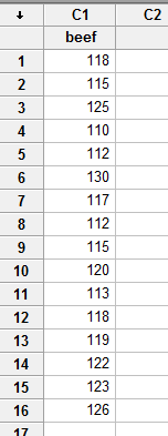
Convince yourself that the data come from a normal distribution... either from your previous experience or by creating a normal probability plot. To ask Minitab to generate a normal probability plot, under the Stat menu, select Basic Statistics, and then select Normality Test...:

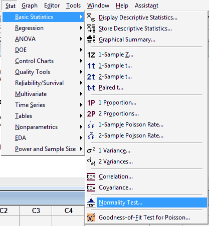
In the pop-up window that appears, select the data (column) to be plotted so that it appears in the box labeled Variable:

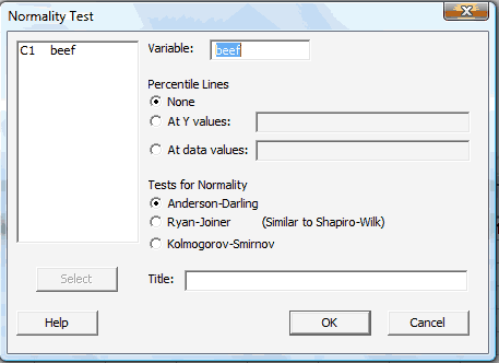
Select OK. When you do so, a new graphics window should appear containing the normal probability plot:

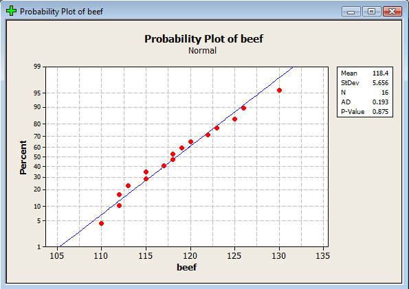
(The plot appearing in the example above was generated in Minitab using different commands. That's why it looks different from this one.)
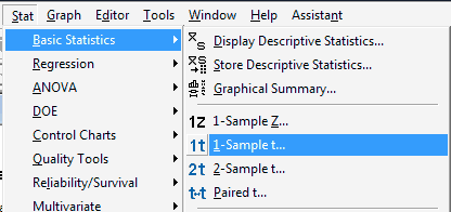
Then, after convincing yourself that the normality assumption is appropriate, under the Stat menu, select Basic Statistics, and then select 1-Sample t...:

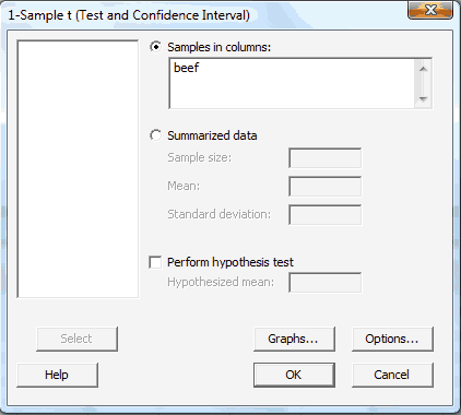
In the pop-up window that appears, select the column (data) to be analyzed so that it appears in the box labeled Samples in columns:
Select OK. The confidence interval output will appear in the Session window. Here is what the Minitab output looks like for the beef example:

One-Sample T: beef

Variable	N	Mean	StDev	SE Mean	95% CI
beef	16	118.44	5.66	1.41	(115.42, 121.45)

2.6 - Non-normal Data

So far, all of our discussion has been on finding a confidence interval for the population mean $\mu$ when the data are normally distributed. That is, the $t$-interval for $\mu$ (and $Z$-interval, for that matter) is derived assuming that the data $X_1, X_2, \ldots, X_n$ are normally distributed. What happens if our data are skewed, and therefore clearly not normally distributed?

Well, it is helpful to note that as the sample size $n$ increases, the $T$ ratio:

$T=\dfrac{\bar{X}-\mu}{\frac{S}{\sqrt{n}}}$

approaches an approximate normal distribution regardless of the distribution of the original data. The implication, therefore, is that the $t$-interval for $\mu$:

$\bar{x}\pm t_{\alpha/2,n-1}\left(\dfrac{s}{\sqrt{n}}\right)$

and the $Z$-interval for $\mu$:

$\bar{x}\pm z_{\alpha/2}\left(\dfrac{s}{\sqrt{n}}\right)$

(with the sample standard deviation s replacing the unknown population standard deviation $\sigma$!) yield similar results for large samples. This result suggests that we should adhere to the following guidelines in practice.

In practice!

Use $\bar{x}\pm t_{\alpha/2,n-1}\left(\dfrac{s}{\sqrt{n}}\right)$ if the data are normally distributed.
If you have reason to believe that the data are not normally distributed, then make sure you have a large enough sample ( $n\ge 30$ generally suffices, but recall that it depends on the skewness of the distribution.) Then:

$\bar{x}\pm t_{\alpha/2,n-1}\left(\dfrac{s}{\sqrt{n}}\right)$ and $\bar{x}\pm z_{\alpha/2}\left(\dfrac{s}{\sqrt{n}}\right)$

will give similar results.
If the data are not normally distributed and you have a small sample, use:

$\bar{x}\pm t_{\alpha/2,n-1}\left(\dfrac{s}{\sqrt{n}}\right)$

with extreme caution and/or use a nonparametric confidence interval for the median (which we'll learn about later in this course).

Example 2-3

A random sample of 64 guinea pigs yielded the following survival times (in days):

36	18	91	89	87	86	52	50	149	120
119	118	115	114	114	108	102	189	178	173
167	167	166	165	160	216	212	209	292	279
278	273	341	382	380	367	355	446	432	421
421	474	463	455	546	545	505	590	576	569
641	638	637	634	621	608	607	603	688	685
663	650	735	725

What is the mean survival time (in days) of the population of guinea pigs? (Data from K. Doksum, Annals of Statistics, 2(1974): 267-277.)

Solution

Because the data points on the normally probability plot do not adhere well to a straight line:

normal probability plot

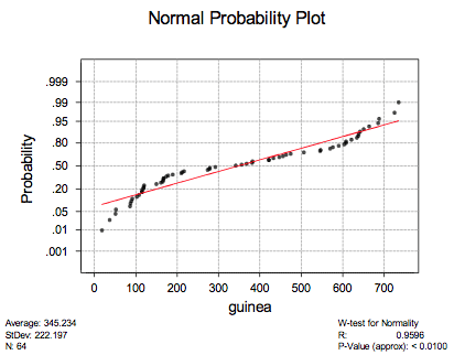
it suggests that the survival times are not normally distributed. We have a large sample though ( $n=64$). Therefore, we should be able to use the $t$-interval for the mean without worry. Asking Minitab to calculate the interval for us, we get:

One-Sample T: guinea

Variable	N	Mean	StDev	SE Mean	95.0% CI
guinea	64	345.2	222.2	27.8	(289.7, 400.7)

That is, we can be 95% confident that the mean survival time for the population of guinea pigs is between 289.7 and 400.7 days.

Incidentally, as the following Minitab output suggests, the $Z$-interval for the mean is quite close to that of the $t$-interval for the mean:

One-Sample Z: guinea

The assumed sigma = 222.2

Variable	N	Mean	StDev	SE Mean	95.0% CI
guinea	64	345.2	222.2	27.8	(290.8, 399.7)

as we would expect, because the sample is quite large.

^[1]	Link
↥	Has Tooltip/Popover
	Toggleable Visibility

Lesson 2: Confidence Intervals for One Mean

Overview

Objectives

2.1 - The Situation

The Problem

A Solution

2.2 - A Z-Interval for a Mean

Example 2-1

Answer

Using Minitab

One-Sample Z

2.3 - Interpretation

2.4 - An Interval's Length

2.5 - A t-Interval for a Mean

Our work so far

What if \(\sigma\) is unknown?

How is \(T=\dfrac{\bar{X}-\mu}{S/\sqrt{n}}\) distributed?

Proof

Proof

Example 2-2

Answer

Minitab^®

Using Minitab

One-Sample T: beef

2.6 - Non-normal Data

In practice!

Example 2-3

Solution

One-Sample T: guinea

One-Sample Z: guinea

The assumed sigma = 222.2

Lesson 2: Confidence Intervals for One Mean

Overview

Objectives

2.1 - The Situation

The Problem

A Solution

2.2 - A Z-Interval for a Mean

Example 2-1

Answer

Using Minitab

One-Sample Z

2.3 - Interpretation

2.4 - An Interval's Length

2.5 - A t-Interval for a Mean

Our work so far

What if \(\sigma\) is unknown?

How is \(T=\dfrac{\bar{X}-\mu}{S/\sqrt{n}}\) distributed?

Proof

Proof

Example 2-2

Answer

Minitab®

Using Minitab

One-Sample T: beef

2.6 - Non-normal Data

In practice!

Example 2-3

Solution

One-Sample T: guinea

One-Sample Z: guinea

The assumed sigma = 222.2

Minitab^®