2.2 - A Z-Interval for a Mean
2.2 - A Z-Interval for a MeanNow that we have a general idea of what a confidence interval is, we'll now turn our attention to deriving a particular confidence interval, namely that of a population mean \(\mu\). We'll jump right ahead to the punch line and then back off and prove the result. But, before stating the result, we need to remind ourselves of a bit of notation.
Recall that the value:
\(z_{\alpha/2}\)
is the \(Z\)-value (obtained from a standard normal table) such that the area to the right of it under the standard normal curve is \(\dfrac{\alpha}{2}\). That is:
\(P(Z\geq z_{\alpha/2})=\alpha/2\)
Likewise:
\(-z_{\alpha/2}\)
is the \(Z\)-value (obtained from a standard normal table) such that the area to the left of it under the standard normal curve is \(\dfrac{\alpha}{2}\). That is:
\(P(Z\leq -z_{\alpha/2})=\alpha/2\)
I like to illustrate this notation with the following diagram of a standard normal curve:
With the notation now recalled, let's state the formula for a confidence interval for the population mean.
-
\(X_1, X_2, \ldots, X_n\) is a random sample from a normal population with mean \(\mu\) and variance \(\sigma^2\). So that:
\(\bar{X}\sim N\left(\mu,\dfrac{\sigma^2}{n}\right)\) and \(Z=\dfrac{\bar{X}-\mu}{\sigma/\sqrt{n}}\sim N(0,1)\)
-
The population variance \(\sigma^2\)is known.
Then, a \((1-\alpha)100\%\) confidence interval for the mean \(\mu\) is:
\(\bar{x}\pm z_{\alpha/2}\left(\dfrac{\sigma}{\sqrt{n}}\right)\)
The interval, because it depends on \(Z\), is often referred to as the \(Z\)-interval for a mean.
Since, at this point, we're just interested in learning the basics of how to derive a confidence interval, we are going to ignore, for now, that the second assumption about the population variance being known is unrealistic. After all, when would we ever think we would know the value of the population variance \(\sigma^2\), but not the population mean \(\mu\)? Go figure! We'll work on finding a practical confidence interval for the mean \(\mu\) later. For now, let's work on deriving this one.
From the above diagram of the standard normal curve, we can see that the following probability statement is true:
\(P[-z_{\alpha/2}\leq Z \leq z_{\alpha/2}]=1-\alpha \)
Then, simply replacing \(Z\), we get:
\(P[-z_{\alpha/2}\leq \dfrac{\bar{X}-\mu}{\sigma/\sqrt{n}} \leq z_{\alpha/2}]=1-\alpha \)
Now, let's focus only on manipulating the inequality inside the brackets for a bit. Because we manipulate each of the three sides of the inequality equally, each of the following statements are equivalent:
\begin{array}{rccl} -z_{\alpha/2} & \leq & \dfrac{\bar{X}-\mu}{\sigma/\sqrt{n}} & \leq & z_{\alpha/2}\\ -z_{\alpha/2}\left(\dfrac{\sigma}{\sqrt{n}}\right) & \leq & \bar{X}-\mu & \leq & +z_{\alpha/2}\left(\dfrac{\sigma}{\sqrt{n}}\right)\\ -\bar{X}-z_{\alpha/2}\left(\dfrac{\sigma}{\sqrt{n}}\right) & \leq & -\mu & \leq & -\bar{X}+z_{\alpha/2}\left(\dfrac{\sigma}{\sqrt{n}}\right)\\ \bar{X}-z_{\alpha/2}\left(\dfrac{\sigma}{\sqrt{n}}\right) & \leq & \mu &\leq & \bar{X}+z_{\alpha/2}\left(\dfrac{\sigma}{\sqrt{n}}\right) \end{array}
So, in summary, by manipulating the inequality, we have shown that the following probability statement is true:
\(P\left[ \bar{X}-z_{\alpha/2}\left(\dfrac{\sigma}{\sqrt{n}}\right) \leq \mu \leq \bar{X}+z_{\alpha/2}\left(\dfrac{\sigma}{\sqrt{n}}\right) \right]=1-\alpha\)
In reality, we'll learn on the next page why we shouldn't (and therefore don't!) write the formula for the \(Z\)-interval for the mean quite like that. Instead, we write that we can be |((1-\alpha)100\%\) confident that the mean \(\mu\) is in the interval:
\(\left[ \bar{x}-z_{\alpha/2}\left(\dfrac{\sigma}{\sqrt{n}}\right), \bar{x}+z_{\alpha/2}\left(\dfrac{\sigma}{\sqrt{n}}\right)\right]\)
Example 2-1

A random sample of 126 police officers subjected to constant inhalation of automobile exhaust fumes in downtown Cairo had an average blood lead level concentration of 29.2 \(\mu g/dl\). Assume \(X\), the blood lead level of a randomly selected policeman, is normally distributed with a standard deviation of \(\sigma=7.5\) \(\mu g/dl\). Historically, it is known that the average blood lead level concentration of humans with no exposure to automobile exhaust is 18.2 \(\mu g/dl\). Is there convincing evidence that policemen exposed to constant auto exhaust have elevated blood lead level concentrations? (Data source: Kamal, Eldamaty, and Faris, "Blood lead level of Cairo traffic policemen," Science of the Total Environment, 105(1991): 165-170.)
Answer
Let's try to answer the question by calculating a 95% confidence interval for the population mean. For a 95% confidence interval, \(1-\alpha=0.95\), so that \(\alpha=0.05\) and \(\dfrac{\alpha}{2}=0.025\). Therefore, as the following diagram illustrates the situation, \(z_{0.025}=1.96\):
Now, substituting in what we know (\(\bar{x}\) = 29.2, \(n=126\), \(\sigma=7.5\), and \(z_{0.025}=1.96\)) into the the formula for a \(Z\)-interval for a mean, we get:
\(\left[29.2-1.96\left(\dfrac{7.5}{\sqrt{126}}\right),29.2+1.96\left(\dfrac{7.5}{\sqrt{126}}\right)\right]\)
Simplifying, we get a 95% confidence interval for the mean blood lead level concentration of all policemen exposed to constant auto exhaust:
\([27.89,30.51]\)
That is, we can be 95% confident that the mean blood lead level concentration of all policemen exposed to constant auto exhaust is between \(27.9 \mu g/dl\) and \(30.5 \mu g/dl\). Note that the interval does not contain the value 18.2, the average blood lead level concentration of humans with no exposure to automobile exhaust. In fact, all of the values in the confidence interval are much greater than 18.2. Therefore, there is convincing evidence that policemen exposed to constant auto exhaust have elevated blood lead level concentrations.
Using Minitab
Statistical software, such as Minitab, can make calculating confidence intervals easier. To ask Minitab to calculate a confidence interval for a mean \(\mu\), with an assumed population standard deviation, you need to do this:
-
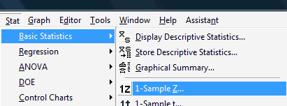
Under the Stat menu, select Basic Statistics, and then select 1-Sample Z...:

The dot-dot-dot (...) that appears after 1-Sample Z is Minitab's way of telling you that you should expect a pop-up window to appear when you click on it.
-
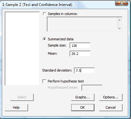
In the pop-up window that does appear, click on the radio button labeled Summarized data. Then, enter the Sample size, Mean, and Standard deviation in the boxes provided. Here's what the completed pop-up window would look like for the example above.

-
Select OK. The confidence interval output will appear in the Session window. Here is what the Minitab output would like for the example above:
One-Sample Z
The assumed standard deviation = 7.5N Mean StDev 95% CI 126 29.2000 0.6682 (27.9804, 30.5096)