Lesson 3: Confidence Intervals for Two Means
Lesson 3: Confidence Intervals for Two MeansObjectives
In this lesson, we derive confidence intervals for the difference in two population means, \(\mu_1-\mu_2\), under three circumstances:
- when the populations are independent and normally distributed with a common variance \(\sigma^2\)
- when the populations are independent and normally distributed with unequal variances
- when the populations are dependent and normally distributed
3.1 - Two-Sample Pooled t-Interval
3.1 - Two-Sample Pooled t-IntervalExample 3-1
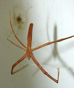
The feeding habits of two species of net-casting spiders are studied. The species, the deinopis and menneus, coexist in eastern Australia. The following data were obtained on the size, in millimeters, of the prey of random samples of the two species:
Size of Random Pray Samples of the Deinopis Spider in Millimeters
| sample 1 | sample 2 | sample 3 | sample 4 | sample 5 | sample 6 | sample 7 | sample 8 | sample 9 | sample 10 |
|---|---|---|---|---|---|---|---|---|---|
| 12.9 | 10.2 | 7.4 | 7.0 | 10.5 | 11.9 | 7.1 | 9.9 | 14.4 | 11.3 |
Size of Random Pray Samples of the Menneus Spider in Millimeters
| sample 1 | sample 2 | sample 3 | sample 4 | sample 5 | sample 6 | sample 7 | sample 8 | sample 9 | sample 10 |
|---|---|---|---|---|---|---|---|---|---|
| 10.2 | 6.9 | 10.9 | 11.0 | 10.1 | 5.3 | 7.5 | 10.3 | 9.2 | 8.8 |
What is the difference, if any, in the mean size of the prey (of the entire populations) of the two species?
Answer
Let's start by formulating the problem in terms of statistical notation. We have two random variables, for example, which we can define as:
- \(X_i\) = the size (in millimeters) of the prey of a randomly selected deinopis spider
- \(Y_i\) = the size (in millimeters) of the prey of a randomly selected menneus spider
In statistical notation, then, we are asked to estimate the difference in the two population means, that is:
\(\mu_X-\mu_Y\)
(By virtue of the fact that the spiders were selected randomly, we can assume the measurements are independent.)
We clearly need some help before we can finish our work on the example. Let's see what the following theorem does for us.
If \(X_1,X_2,\ldots,X_n\sim N(\mu_X,\sigma^2)\) and \(Y_1,Y_2,\ldots,Y_m\sim N(\mu_Y,\sigma^2)\) are independent random samples, then a \((1-\alpha)100\%\) confidence interval for \(\mu_X-\mu_Y\), the difference in the population means is:
\((\bar{X}-\bar{Y})\pm (t_{\alpha/2,n+m-2}) S_p \sqrt{\dfrac{1}{n}+\dfrac{1}{m}}\)
where \(S_p^2\), the "pooled sample variance":
\(S_p^2=\dfrac{(n-1)S^2_X+(m-1)S^2_Y}{n+m-2}\)
is an unbiased estimator of the common variance \(\sigma^2\).
Proof
We'll start with the punch line first. If it is known that:
\(T=\dfrac{(\bar{X}-\bar{Y})-(\mu_X-\mu_Y)}{S_p\sqrt{\dfrac{1}{n}+\dfrac{1}{m}}} \sim t_{n+m-2}\)
then the proof is a bit on the trivial side, because we then know that:
\(P\left[-t_{\alpha/2,n+m-2} \leq \dfrac{(\bar{X}-\bar{Y})-(\mu_X-\mu_Y)}{S_p\sqrt{\dfrac{1}{n}+\dfrac{1}{m}}} \leq t_{\alpha/2,n+m-2}\right]=1-\alpha\)
And then, it is just a matter of manipulating the inequalities inside the parentheses. First, multiplying through the inequality by the quantity in the denominator, we get:
\(-t_{\alpha/2,n+m-2}\times S_p\sqrt{\dfrac{1}{n}+\dfrac{1}{m}} \leq (\bar{X}-\bar{Y})-(\mu_X-\mu_Y)\leq t_{\alpha/2,n+m-2}\times S_p\sqrt{\dfrac{1}{n}+\dfrac{1}{m}}\)
Then, subtracting through the inequality by the difference in the sample means, we get:
\(-(\bar{X}-\bar{Y})-t_{\alpha/2,n+m-2}\times S_p\sqrt{\dfrac{1}{n}+\dfrac{1}{m}} \leq -(\mu_X-\mu_Y) \leq -(\bar{X}-\bar{Y})+t_{\alpha/2,n+m-2}\times S_p\sqrt{\dfrac{1}{n}+\dfrac{1}{m}} \)
And, finally, dividing through the inequality by −1, and thereby changing the direction of the inequality signs, we get:
\((\bar{X}-\bar{Y})-t_{\alpha/2,n+m-2}\times S_p\sqrt{\dfrac{1}{n}+\dfrac{1}{m}} \leq \mu_X-\mu_Y \leq (\bar{X}-\bar{Y})+t_{\alpha/2,n+m-2}\times S_p\sqrt{\dfrac{1}{n}+\dfrac{1}{m}} \)
That is, we get the claimed \((1-\alpha)100\%\) confidence interval for the difference in the population means:
\((\bar{X}-\bar{Y})\pm (t_{\alpha/2,n+m-2}) S_p \sqrt{\dfrac{1}{n}+\dfrac{1}{m}}\)
Now, it's just a matter of going back and proving that first distributional result, namely that:
\(T=\dfrac{(\bar{X}-\bar{Y})-(\mu_X-\mu_Y)}{S_p\sqrt{\dfrac{1}{n}+\dfrac{1}{m}}} \sim t_{n+m-2}\)
Well, by the assumed normality of the \(X_i\) and \(Y_i\) measurements, we know that the means of each of the samples are also normally distributed. That is:
\(\bar{X}\sim N \left(\mu_X,\dfrac{\sigma^2}{n}\right)\) and \(\bar{Y}\sim N \left(\mu_Y,\dfrac{\sigma^2}{m}\right)\)
Then, the independence of the two samples implies that the difference in the two sample means is normally distributed with the mean equaling the difference in the two population means and the variance equaling the sum of the two variances. That is:
\(\bar{X}-\bar{Y} \sim N\left(\mu_X-\mu_Y,\dfrac{\sigma^2}{n}+\dfrac{\sigma^2}{m}\right)\)
Now, we can standardize the difference in the two sample means to get:
\(Z=\dfrac{(\bar{X}-\bar{Y})-(\mu_X-\mu_Y)}{\sqrt{\dfrac{\sigma^2}{n}+\dfrac{\sigma^2}{m}}} \sim N(0,1)\)
Now, the normality of the \(X_i\) and \(Y_i\) measurements also implies that:
\(\dfrac{(n-1)S^2_X}{\sigma^2}\sim \chi^2_{n-1}\) and \(\dfrac{(m-1)S^2_Y}{\sigma^2}\sim \chi^2_{m-1}\)
And, the independence of the two samples implies that when we add those two chi-square random variables, we get another chi-square random variable with the degrees of freedom (\(n-1\) and \(m-1\)) added. That is:
\(U=\dfrac{(n-1)S^2_X}{\sigma^2}+\dfrac{(m-1)S^2_Y}{\sigma^2}\sim \chi^2_{n+m-2}\)
Now, it's just a matter of using the definition of a \(T\)-random variable:
\(T=\dfrac{Z}{\sqrt{U/(n+m-2)}}\)
Substituting in the values we defined above for \(Z\) and \(U\), we get:
\(T=\dfrac{\dfrac{(\bar{X}-\bar{Y})-(\mu_X-\mu_Y)}{\sqrt{\dfrac{\sigma^2}{n}+\dfrac{\sigma^2}{m}}}}{\sqrt{\left[\dfrac{(n-1)S^2_X}{\sigma^2}+\dfrac{(m-1)S^2_Y}{\sigma^2}\right]/(n+m-2)}}\)
Pulling out a factor of \(\frac{1}{\sigma}\) in both the numerator and denominator, we get:
\(T=\dfrac{\dfrac{1}{\sigma} \dfrac{(\bar{X}-\bar{Y})-(\mu_X-\mu_Y)}{\sqrt{\dfrac{1}{n}+\dfrac{1}{m}}}}{\dfrac{1}{\sigma} \sqrt{\dfrac{(n-1)S^2_X+(m-1)S^2_Y}{(n+m-2)}}}\)
And, canceling out the \(\frac{1}{\sigma}\)'s and recognizing that the denominator is the pooled standard deviation, \(S_p\), we get:
\(T=\dfrac{(\bar{X}-\bar{Y})-(\mu_X-\mu_Y)}{S_p\sqrt{\dfrac{1}{n}+\dfrac{1}{m}}}\)
That is, we have shown that:
\(T=\dfrac{(\bar{X}-\bar{Y})-(\mu_X-\mu_Y)}{S_p\sqrt{\dfrac{1}{n}+\dfrac{1}{m}}}\sim t_{n+m-2}\)
And we are done.... our proof is complete!
Note!
-
Three assumptions are made in deriving the above confidence interval formula. They are:
- The measurements ( \(X_i\) and \(Y_i\)) are independent.
- The measurements in each population are normally distributed.
- The measurements in each population have the same variance \(\sigma^2\).
That means that we should use the interval to estimate the difference in two population means only when the three conditions hold for our given data set. Otherwise, the confidence interval wouldn't be an accurate estimate of the difference in the two population means.
-
There are no restrictions on the sample sizes \(n\) and \(m\). They don't have to be equal and they don't have to be large.
-
The pooled sample variance \(S_p^2\) is an average of the sample variances weighted by their sample sizes. The larger sample size gets more weight. For example, suppose:
\(n=11\) and \(m=31\)
\(s^2_x=4\) and \(s^2_y=8\)
Then, the unweighted average of the sample variances is 6, as shown here:
\(\dfrac{4+8}{2}=6\)
But, the pooled sample variance is 7, as the following calculation illustrates:
\(s_p^2=\dfrac{(11-1)4+(31-1)8}{11+31-2}=\dfrac{10(4)+30(8)}{40}=7\)
In this case, the larger sample size (\(m=31\)) is associated with the variance of 8, and so the pooled sample variance get "pulled" upwards from the unweighted average of 6 to the weighted average of 7. By the way, note that if the sample sizes are equal, that is, \(m=n=r\), say, then the pooled sample variance \(S_p^2\) reduces to an unweighted average.
With all of the technical details behinds us, let's now return to our example.
Example 3-1 (Continued)
The feeding habits of two species of net-casting spiders are studied. The species, the deinopis and menneus, coexist in eastern Australia. The following data were obtained on the size, in millimeters, of the prey of random samples of the two species:
Size of Random Pray Samples of the Deinopis Spider in Millimeters
| sample 1 | sample 2 | sample 3 | sample 4 | sample 5 | sample 6 | sample 7 | sample 8 | sample 9 | sample 10 |
|---|---|---|---|---|---|---|---|---|---|
| 12.9 | 10.2 | 7.4 | 7.0 | 10.5 | 11.9 | 7.1 | 9.9 | 14.4 | 11.3 |
Size of Random Pray Samples of the Menneus Spider in Millimeters
| sample 1 | sample 2 | sample 3 | sample 4 | sample 5 | sample 6 | sample 7 | sample 8 | sample 9 | sample 10 |
|---|---|---|---|---|---|---|---|---|---|
| 10.2 | 6.9 | 10.9 | 11.0 | 10.1 | 5.3 | 7.5 | 10.3 | 9.2 | 8.8 |
What is the difference, if any, in the mean size of the prey (of the entire populations) of the two species?
Answer
First, we should make at least a superficial attempt to address whether the three conditions are met. Given that the data were obtained in a random manner, we can go ahead and believe that the condition of independence is met. Given that the sample variances are not all that different, that is, they are at least similar in magnitude:
\(s^2_{\text{deinopis}}=6.3001\) and \(s^2_{\text{menneus}}=3.61\)
we can go ahead and assume that the variances of the two populations are similar. Assessing normality is a bit trickier, as the sample sizes are quite small. Let me just say that normal probability plots don't give an alarming reason to rule out the possibility that the measurements are normally distributed. So, let's proceed!
The pooled sample variance is calculated to be 4.955:
\(s_p^2=\dfrac{(10-1)6.3001+(10-1)3.61}{10+10-2}=4.955\)
which leads to a pooled standard deviation of 2.226:
\(s_p=\sqrt{4.955}=2.226\)
(Of course, because the sample sizes are equal (\(m=n=10\)), the pooled sample variance is just an unweighted average of the two variances 6.3001 and 3.61).
Because \(m=n=10\), if we were to calculate a 95% confidence interval for the difference in the two means, we need to use a \(t\)-table or statistical software to determine that:
\(t_{0.025,10+10-2}=t_{0.025,18}=2.101\)
The sample means are calculated to be:
\(\bar{x}_{\text{deinopis}}=10.26\) and \(\bar{y}_{\text{menneus}}=9.02\)
We have everything we need now to calculate a 95% confidence interval for the difference in the population means. It is:
\((10.26-9.02)\pm 2.101(2.226)\sqrt{\dfrac{1}{10}+\dfrac{1}{10}}\)
which simplifies to:
\(1.24 \pm 2.092\) or \((-0.852,3.332)\)
That is, we can be 95% confident that the actual mean difference in the size of the prey is between −0.85 mm and 3.33 mm. Because the interval contains the value 0, we cannot conclude that the population means differ.
Minitab®
Using Minitab
The commands necessary for asking Minitab to calculate a two-sample pooled \(t\)-interval for \(\mu_x-\mu_y\) depend on whether the data are entered in two columns, or the data are entered in one column with a grouping variable in a second column. We'll illustrate using the spider and prey example.
- Step 1
Enter the data in two columns, such as:

- Step 2
Under the Stat menu, select Basic Statistics, and then select 2-Sample t...:
- Step 3
In the pop-up window that appears, select Samples in different columns. Specify the name of the First variable, and specify the name of the Second variable. Click on the box labeled Assume equal variances. (If you want a confidence level that differs from Minitab's default level of 95.0, under Options..., type in the desired confidence level. Select Ok on the Options window.) Select Ok on the 2-Sample t... window:
When the Data are Entered in Two Columns
The confidence interval output will appear in the session window. Here's what the output looks like for the spider and prey example with the confidence interval circled in red:
Two-Sample T For Deinopis vs Menneus
| Variable | N | Mean | StDev | SE Mean |
|---|---|---|---|---|
| Deinopis | 10 | 10.26 | 2.51 | 0.79 |
| Menneus | 10 | 9.02 | 1.90 | 0.60 |
Difference = mu (Deinopis) - mu (Menneus)
Estimate for difference: 1.240
95% CI for difference: (-0.852, 3.332)
T-Test of difference = 0 (vs not =): T-Value = 1.25 P-Value = 0.229 DF = 18
Both use Pooled StDev = 2.2266
When the Data are Entered in One Column, and a Grouping Variable in a Second Column
- Step 1
Enter the data in one column (called Prey, say), and the grouping variable in a second column (called Group, say, with 1 denoting a deinopis spider and 2 denoting a menneus spider), such as:
- Step 2
Under the Stat menu, select Basic Statistics, and then select 2-Sample t...:
- Step 3
In the pop-up window that appears, select Samples in one column. Specify the name of the Samples variable (Prey, for us) and specify the name of the Subscripts (grouping) variable (Group, for us). Click on the box labeled Assume equal variances. (If you want a confidence level that differs from Minitab's default level of 95.0, under Options..., type in the desired confidence level. Select Ok on the Options window.) Select Ok on the 2-sample t... window.
The confidence interval output will appear in the session window. Here's what the output looks like for the example above with the confidence interval circled in red:
Two-Sample T For Prey
| Group | N | Mean | StDev | SE Mean |
|---|---|---|---|---|
| 1 | 10 | 10.26 | 2.51 | 0.79 |
| 2 | 10 | 9.02 | 1.90 | 0.60 |
Difference = mu (1) - mu (2)
Estimate for difference: 1.240
95% CI for difference: (-0.852, 3.332)
T-Test of difference = 0 (vs not =): T-Value = 1.25 P-Value = 0.229 DF = 18
Both use Pooled StDev = 2.2266
3.2 - Welch's t-Interval
3.2 - Welch's t-IntervalIf we want to use the two-sample pooled \(t\)-interval as a way of creating an interval estimate for \(\mu_x-\mu_y\), the difference in the means of two independent populations, then we must be confident that the population variances \(\sigma^2_X\) and \(\sigma^2_Y\) are equal. What do we do though if we can't assume the variances \(\sigma^2_X\) and \(\sigma^2_Y\) are equal? That is, what if \(\sigma^2_X \neq \sigma^2_Y\)? If that's the case, we'll want to use what is typically called Welch's \(t\)-interval.
- Welch's \(t\)-interval
-
Welch's \(t\)-interval for \(\mu_X-\mu_Y\). If:
the data are normally distributed (or if not, the underlying distributions are not too badly skewed, and \(n\) and \(m\) are large enough), and the population variances \(\sigma^2_X\) and \(\sigma^2_Y\) can't be assumed to be equal,then, a \((1-\alpha)100\%\) confidence interval for \(\mu_X-\mu_Y\), the difference in the population means is:
\(\bar{X}-\bar{Y}\pm t_{\alpha/2,r}\sqrt{\dfrac{s^2_X}{n}+\dfrac{s^2_Y}{m}}\)
where the \(r\) degrees of freedom are approximated by:
\(r=\dfrac{\left(\dfrac{s^2_X}{n}+\dfrac{s^2_Y}{m}\right)^2}{\dfrac{(s^2_X/n)^2}{n-1}+\dfrac{(s^2_Y/m)^2}{m-1}}\)
If necessary, as is typically the case, take the integer portion of \(r\), that is, use \([r]\).
Let's take a look at an example.
Example 3-1 (Continuted)
Let's return to the example, in which the feeding habits of two-species of net-casting spiders are studied. The species, the deinopis and menneus, coexist in eastern Australia. The following summary statistics were obtained on the size, in millimeters, of the prey of the two species:
| Adult DEINOPIS | Adult MENNEUS |
|---|---|
| \(n\) = 10 | \(m\) = 10 |
| \(\bar{x}\) = 10.26 mm | \(\bar{y}\) = 9.02 mm |
| \({s^2_X}\)= \((2.51)^2\) | \({s^2_Y}\) = \((1.90)^2\) |
What is the difference in the mean sizes of the prey (of the entire populations) of the two species?
Answer
Hmmm... do those sample variances differ enough to lead us to believe that the population variances differ? If so, we should use Welch's \(t\)-interval instead of the two-sample pooled \(t\)-interval in estimating \(\mu_X-\mu_Y\). Let's calculate Welch's \(t\)-interval to see what we get. Substituting in what we know, the degrees of freedom are calculated as:
\(r=\dfrac{(s^2_X/n+s^2_Y/m)^2}{\dfrac{(s^2_X/n)^2}{n-1}+\dfrac{(s^2_Y/m)^2}{m-1}}=\dfrac{((2.51)^2/10+(1.90)^2/10)^2}{\frac{((2.51)^2/10)^2}{9}+\frac{((1.90)^2/10)^2}{9}}=16.76\)
Because \(r\) is not an integer, we'll take just the integer portion of \(r\), that is, we'll use:
\([r]=16\)
degrees of freedom. Then, using a \(t\)-table (or alternatively, statistical software such as Minitab), we get:
\(t_{0.025,16}=2.120\)
Now, substituting the sample means, sample variances, and sample sizes into the formula for Welch's \(t\)-interval:
\(\bar{X}-\bar{Y}\pm t_{\alpha/2,r}\sqrt{\dfrac{s^2_X}{n}+\dfrac{s^2_Y}{m}}\)
we get:
\((10.26-9.02)\pm 2.120 \sqrt{\dfrac{(2.51)^2}{10}+\dfrac{(1.90)^2}{10}}\)
Simplifying, we get that a 95% confidence interval for \(\mu_X-\mu_Y\) is:
\((-0.870,3.350)\)
We can be 95% confident that the difference in the mean prey size of the two species is between −0.87 and 3.35 mm. Hmmm... you might recall that our two-sample pooled \(t\)-interval was (−0.852, 3.332). Comparing the two intervals, we see that they aren't a whole lot different. That's because the sample variances aren't really all that different. Many statisticians follow the rule of thumb that if the ratio of the two sample variances exceeds 4, that is, if:
either \(\dfrac{s^2_X}{s^2_Y}>4\) or \(\dfrac{s^2_Y}{s^2_X}>4\)
then they'll use Welch's \(t\)-interval for estimating \(\mu_X-\mu_Y\). Otherwise, they'll use the two-sample pooled \(t\)-interval.
Minitab®
Using Minitab
Asking Minitab to calculate Welch's \(t\)-interval for \(\mu_X-\mu_Y\) require just a minor modification to the commands used in asking Minitab to calculate a two-sample pooled \(t\)-interval. We simply skip the step in which we click on the box Assume equal variances. Again, the commands required depend on whether the data are entered in two columns, or the data are entered in one column with a grouping variable in a second column. Since we've already learned how to ask Minitab to calculate a confidence interval for \(\mu_X-\mu_Y\) for both of those data arrangements, we'll take a look instead at the case in which the data are already summarized for us, as they are in the spider and prey example above.
When the Data are Summarized
- Step 1
Under the Stat menu, select Basic Statistics, and then select 2-Sample t...:
- Step 2
In the pop-up window that appears, select Summarized data. Then, for the First variable (deinopis data, for us), type the Sample size, Mean, and Standard deviation in the appropriate boxes. Do the same thing for the Second variable (menneus data, for us), that is, type the Sample size, Mean, and Standard deviation in the appropriate boxes. Select Ok:
The confidence interval output will appear in the session window. Here's what the output looks like for the spider and prey example with the confidence interval circled in red:
Two-Sample T-Test and CI
| Sample | N | Mean | StDev | SE Mean |
|---|---|---|---|---|
| 1 | 10 | 10.26 | 2.51 | 0.79 |
| 2 | 10 | 9.02 | 1.90 | 0.60 |
Difference = mu (1) - mu (2)
Estimate for difference: 1.240
95% CI for difference: (-0.870, 3.350)
T-Test of difference = 0 (vs not =): T-Value = 1.25 P-Value = 0.231 DF = 16
3.3 - Paired t-Interval
3.3 - Paired t-IntervalExample 3-2

Are there physiological indicators associated with schizophrenia? In a 1990 article, researchers reported the results of a study that controlled for genetic and socioeconomic differences by examining 15 pairs of identical twins, where one of the twins was schizophrenic and the other not. The researchers used magnetic resonance imaging to measure the volumes (in cubic centimeters) of several regions and subregions inside the twins' brains. The following data came from one of the subregions, the left hippocampus:
What is the magnitude of the difference in the volumes of the left hippocampus between (all) unaffected and affected individuals?
| Pair | Unaffect | Affect |
|---|---|---|
| 1 | 1.94 | 1.27 |
| 2 | 1.44 | 1.63 |
| 3 | 1.56 | 1.47 |
| 4 | 1.58 | 1.39 |
| 5 | 2.06 | 1.93 |
| 6 | 1.66 | 1.26 |
| 7 | 1.75 | 1.71 |
| 8 | 1.77 | 1.67 |
| 9 | 1.78 | 1.28 |
| 10 | 1.92 | 1.85 |
| 11 | 1.25 | 1.02 |
| 12 | 1.93 | 1.34 |
| 13 | 2.04 | 2.02 |
| 14 | 1.62 | 1.59 |
| 15 | 2.08 | 1.97 |
Answer
Let \(X_i\) (labeled Unaffect) denote the volume of the left hippocampus of unaffected individual \(i\), and let \(Y_i\) (labeled Affect) denote the volume of the left hippocampus of affected individual \(i\). Then, we are interested in finding a confidence interval for the difference of the means:
\(\mu_X-\mu_Y\)
If the pairs of measurements were independent, the calculation of the confidence interval would be trivial, as we could calculate either a pooled two-sample \(t\)-interval or a Welch's \(t\)-interval depending on whether or not we could assume the population variances were equal. But, alas, the \(X_i\) and \(Y_i\) measurements are not independent, since they are measured on the same pair \(i\) of twins! So we can skip that idea of using either of the intervals we've learned so far in this lesson.
Fortunately, though, the calculation of the confidence interval is still trivial! The difference in the measurements of the unaffected and affected individuals, that is:
\(D_i=X_i-Y_i\)
removes the twin effect and therefore quantifies the direct effect of schizophrenia for each (independent) pair \(i\) of twins. In that case, then, we are interested in estimating the mean difference, that is:
\(\mu_D=\mu_X-\mu_Y\)
That is, we have reduced the problem to that of a single population of measurements, which just so happen to be independent differences. Then, we're right back to the situation in which we can use the one-sample \(t\)-interval to estimate \(\mu_D\). We just have to take the extra step of calculating the differences (labeled DiffU−A):
Then, the formula for a 95% confidence interval for \(\mu_D\) is:
\(\bar{d} \pm t_{0.025,14}\left(\dfrac{s_d}{\sqrt{n}}\right)\)
Summarizing the difference data, and consulting a \(t\)-table, we get:
\(0.1987 \pm 2.1448 \left(\dfrac{0.2383}{\sqrt{15}}\right)\)
which simplifies to this:
\(0.1987 \pm 2.1448(0.0615)\)
and this:
\(0.1987 \pm 0.1319\)
and finally this:
\((0.0668,0.3306)\)
| Pair | Unaffect | Affect | DiffU-A |
|---|---|---|---|
| 1 | 1.94 | 1.27 | 0.67 |
| 2 | 1.44 | 1.63 | -0.19 |
| 3 | 1.56 | 1.47 | 0.09 |
| 4 | 1.58 | 1.39 | 0.19 |
| 5 | 2.06 | 1.93 | 0.13 |
| 6 | 1.66 | 1.26 | 0.40 |
| 7 | 1.75 | 1.71 | 0.04 |
| 8 | 1.77 | 1.67 | 0.10 |
| 9 | 1.78 | 1.28 | 0.50 |
| 10 | 1.92 | 1.85 | 0.07 |
| 11 | 1.25 | 1.02 | 0.23 |
| 12 | 1.93 | 1.34 | 0.59 |
| 13 | 2.04 | 2.02 | 0.02 |
| 14 | 1.62 | 1.59 | 0.03 |
| 15 | 2.08 | 1.97 | 0.11 |
That is, we can be 95% confident that the mean size for unaffected individuals is between 0.067 and 0.331 cubic centimeters larger than the mean size for affected individuals.
Let's summarize the method we used in deriving a confidence interval for the difference in the means of two dependent populations.
Result.
In general, when dealing with pairs of dependent measurements, we should use \(\bar{d}\), the sample mean difference, to estimate \(\mu_D\), the population mean difference. As long as the differences are normally distributed, we should use the \((1-\alpha)100\%\) \(t\)-interval for the mean, but now treating the differences as the sample data:
\(\bar{d} \pm t_{\alpha/2,n-1}\left(\dfrac{s_d}{\sqrt{n}}\right)\)
Minitab®
Using Minitab
We've already learned how to use Minitab to calculate a \(t\)-interval for a mean, namely under the Stat menu, select Basic Statistics and then 1-Sample t...:
In calculating a paired t-interval, though, we have to take one additional step, namely that of calculating the differences. First, label an empty column in the worksheet that will contain the differences, DiffU-A, say. Then, under the Calc menu, select Calculator...:
In the pop-up window that appears, click on the box labeled Store result in variable, and then in the left box containing the names of your worksheet columns, double-click on the column labeled as DiffU-A. Then, click on the box labeled Expression, and use the calculator to tell Minitab to take the differences between the relevant columns, Unaffect and Affect, here:
When you click on OK, the output will appear in the Session window, looking something like this, with the 95% confidence interval circled in red:
One-Sample T: DiffU-A
| Variable | N | Mean | StDev | SE Mean | 95.0% CI |
|---|---|---|---|---|---|
| DiffU-A | 15 | 0.1987 | 0.2383 | 0.0615 | ( 0.0667, 0.3306) |
Common Uses of the Paired t-Interval
In the previous example, measurements were taken on one person who was similar in some way with another person, using a design procedure known as matching. That is just one way in which data can be considered "paired." The most common ways in which data can be paired are:
-
A person is matched with a similar person. For example, a person is matched to another person with a similar intelligence (IQ scores, for example) to compare the effects of two educational programs on test scores.
-
Before and after studies. For example, a person is weighed, and then put on a diet, and weighed again.
-
A person serves as his or her own control. For example, a person takes an asthma drug called GoodLungs to assess the improvement on lung function, has a period of 8-weeks in which no drugs are taken (known as a washout period), and then takes a second asthma drug called EvenBetterLungs to again assess the improvement on lung function.