3.1 - Two-Sample Pooled t-Interval
3.1 - Two-Sample Pooled t-IntervalExample 3-1
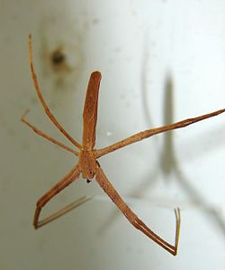
The feeding habits of two species of net-casting spiders are studied. The species, the deinopis and menneus, coexist in eastern Australia. The following data were obtained on the size, in millimeters, of the prey of random samples of the two species:
Size of Random Pray Samples of the Deinopis Spider in Millimeters
| sample 1 | sample 2 | sample 3 | sample 4 | sample 5 | sample 6 | sample 7 | sample 8 | sample 9 | sample 10 |
|---|---|---|---|---|---|---|---|---|---|
| 12.9 | 10.2 | 7.4 | 7.0 | 10.5 | 11.9 | 7.1 | 9.9 | 14.4 | 11.3 |
Size of Random Pray Samples of the Menneus Spider in Millimeters
| sample 1 | sample 2 | sample 3 | sample 4 | sample 5 | sample 6 | sample 7 | sample 8 | sample 9 | sample 10 |
|---|---|---|---|---|---|---|---|---|---|
| 10.2 | 6.9 | 10.9 | 11.0 | 10.1 | 5.3 | 7.5 | 10.3 | 9.2 | 8.8 |
What is the difference, if any, in the mean size of the prey (of the entire populations) of the two species?
Answer
Let's start by formulating the problem in terms of statistical notation. We have two random variables, for example, which we can define as:
- \(X_i\) = the size (in millimeters) of the prey of a randomly selected deinopis spider
- \(Y_i\) = the size (in millimeters) of the prey of a randomly selected menneus spider
In statistical notation, then, we are asked to estimate the difference in the two population means, that is:
\(\mu_X-\mu_Y\)
(By virtue of the fact that the spiders were selected randomly, we can assume the measurements are independent.)
We clearly need some help before we can finish our work on the example. Let's see what the following theorem does for us.
If \(X_1,X_2,\ldots,X_n\sim N(\mu_X,\sigma^2)\) and \(Y_1,Y_2,\ldots,Y_m\sim N(\mu_Y,\sigma^2)\) are independent random samples, then a \((1-\alpha)100\%\) confidence interval for \(\mu_X-\mu_Y\), the difference in the population means is:
\((\bar{X}-\bar{Y})\pm (t_{\alpha/2,n+m-2}) S_p \sqrt{\dfrac{1}{n}+\dfrac{1}{m}}\)
where \(S_p^2\), the "pooled sample variance":
\(S_p^2=\dfrac{(n-1)S^2_X+(m-1)S^2_Y}{n+m-2}\)
is an unbiased estimator of the common variance \(\sigma^2\).
Proof
We'll start with the punch line first. If it is known that:
\(T=\dfrac{(\bar{X}-\bar{Y})-(\mu_X-\mu_Y)}{S_p\sqrt{\dfrac{1}{n}+\dfrac{1}{m}}} \sim t_{n+m-2}\)
then the proof is a bit on the trivial side, because we then know that:
\(P\left[-t_{\alpha/2,n+m-2} \leq \dfrac{(\bar{X}-\bar{Y})-(\mu_X-\mu_Y)}{S_p\sqrt{\dfrac{1}{n}+\dfrac{1}{m}}} \leq t_{\alpha/2,n+m-2}\right]=1-\alpha\)
And then, it is just a matter of manipulating the inequalities inside the parentheses. First, multiplying through the inequality by the quantity in the denominator, we get:
\(-t_{\alpha/2,n+m-2}\times S_p\sqrt{\dfrac{1}{n}+\dfrac{1}{m}} \leq (\bar{X}-\bar{Y})-(\mu_X-\mu_Y)\leq t_{\alpha/2,n+m-2}\times S_p\sqrt{\dfrac{1}{n}+\dfrac{1}{m}}\)
Then, subtracting through the inequality by the difference in the sample means, we get:
\(-(\bar{X}-\bar{Y})-t_{\alpha/2,n+m-2}\times S_p\sqrt{\dfrac{1}{n}+\dfrac{1}{m}} \leq -(\mu_X-\mu_Y) \leq -(\bar{X}-\bar{Y})+t_{\alpha/2,n+m-2}\times S_p\sqrt{\dfrac{1}{n}+\dfrac{1}{m}} \)
And, finally, dividing through the inequality by −1, and thereby changing the direction of the inequality signs, we get:
\((\bar{X}-\bar{Y})-t_{\alpha/2,n+m-2}\times S_p\sqrt{\dfrac{1}{n}+\dfrac{1}{m}} \leq \mu_X-\mu_Y \leq (\bar{X}-\bar{Y})+t_{\alpha/2,n+m-2}\times S_p\sqrt{\dfrac{1}{n}+\dfrac{1}{m}} \)
That is, we get the claimed \((1-\alpha)100\%\) confidence interval for the difference in the population means:
\((\bar{X}-\bar{Y})\pm (t_{\alpha/2,n+m-2}) S_p \sqrt{\dfrac{1}{n}+\dfrac{1}{m}}\)
Now, it's just a matter of going back and proving that first distributional result, namely that:
\(T=\dfrac{(\bar{X}-\bar{Y})-(\mu_X-\mu_Y)}{S_p\sqrt{\dfrac{1}{n}+\dfrac{1}{m}}} \sim t_{n+m-2}\)
Well, by the assumed normality of the \(X_i\) and \(Y_i\) measurements, we know that the means of each of the samples are also normally distributed. That is:
\(\bar{X}\sim N \left(\mu_X,\dfrac{\sigma^2}{n}\right)\) and \(\bar{Y}\sim N \left(\mu_Y,\dfrac{\sigma^2}{m}\right)\)
Then, the independence of the two samples implies that the difference in the two sample means is normally distributed with the mean equaling the difference in the two population means and the variance equaling the sum of the two variances. That is:
\(\bar{X}-\bar{Y} \sim N\left(\mu_X-\mu_Y,\dfrac{\sigma^2}{n}+\dfrac{\sigma^2}{m}\right)\)
Now, we can standardize the difference in the two sample means to get:
\(Z=\dfrac{(\bar{X}-\bar{Y})-(\mu_X-\mu_Y)}{\sqrt{\dfrac{\sigma^2}{n}+\dfrac{\sigma^2}{m}}} \sim N(0,1)\)
Now, the normality of the \(X_i\) and \(Y_i\) measurements also implies that:
\(\dfrac{(n-1)S^2_X}{\sigma^2}\sim \chi^2_{n-1}\) and \(\dfrac{(m-1)S^2_Y}{\sigma^2}\sim \chi^2_{m-1}\)
And, the independence of the two samples implies that when we add those two chi-square random variables, we get another chi-square random variable with the degrees of freedom (\(n-1\) and \(m-1\)) added. That is:
\(U=\dfrac{(n-1)S^2_X}{\sigma^2}+\dfrac{(m-1)S^2_Y}{\sigma^2}\sim \chi^2_{n+m-2}\)
Now, it's just a matter of using the definition of a \(T\)-random variable:
\(T=\dfrac{Z}{\sqrt{U/(n+m-2)}}\)
Substituting in the values we defined above for \(Z\) and \(U\), we get:
\(T=\dfrac{\dfrac{(\bar{X}-\bar{Y})-(\mu_X-\mu_Y)}{\sqrt{\dfrac{\sigma^2}{n}+\dfrac{\sigma^2}{m}}}}{\sqrt{\left[\dfrac{(n-1)S^2_X}{\sigma^2}+\dfrac{(m-1)S^2_Y}{\sigma^2}\right]/(n+m-2)}}\)
Pulling out a factor of \(\frac{1}{\sigma}\) in both the numerator and denominator, we get:
\(T=\dfrac{\dfrac{1}{\sigma} \dfrac{(\bar{X}-\bar{Y})-(\mu_X-\mu_Y)}{\sqrt{\dfrac{1}{n}+\dfrac{1}{m}}}}{\dfrac{1}{\sigma} \sqrt{\dfrac{(n-1)S^2_X+(m-1)S^2_Y}{(n+m-2)}}}\)
And, canceling out the \(\frac{1}{\sigma}\)'s and recognizing that the denominator is the pooled standard deviation, \(S_p\), we get:
\(T=\dfrac{(\bar{X}-\bar{Y})-(\mu_X-\mu_Y)}{S_p\sqrt{\dfrac{1}{n}+\dfrac{1}{m}}}\)
That is, we have shown that:
\(T=\dfrac{(\bar{X}-\bar{Y})-(\mu_X-\mu_Y)}{S_p\sqrt{\dfrac{1}{n}+\dfrac{1}{m}}}\sim t_{n+m-2}\)
And we are done.... our proof is complete!
Note!
-
Three assumptions are made in deriving the above confidence interval formula. They are:
- The measurements ( \(X_i\) and \(Y_i\)) are independent.
- The measurements in each population are normally distributed.
- The measurements in each population have the same variance \(\sigma^2\).
That means that we should use the interval to estimate the difference in two population means only when the three conditions hold for our given data set. Otherwise, the confidence interval wouldn't be an accurate estimate of the difference in the two population means.
-
There are no restrictions on the sample sizes \(n\) and \(m\). They don't have to be equal and they don't have to be large.
-
The pooled sample variance \(S_p^2\) is an average of the sample variances weighted by their sample sizes. The larger sample size gets more weight. For example, suppose:
\(n=11\) and \(m=31\)
\(s^2_x=4\) and \(s^2_y=8\)
Then, the unweighted average of the sample variances is 6, as shown here:
\(\dfrac{4+8}{2}=6\)
But, the pooled sample variance is 7, as the following calculation illustrates:
\(s_p^2=\dfrac{(11-1)4+(31-1)8}{11+31-2}=\dfrac{10(4)+30(8)}{40}=7\)
In this case, the larger sample size (\(m=31\)) is associated with the variance of 8, and so the pooled sample variance get "pulled" upwards from the unweighted average of 6 to the weighted average of 7. By the way, note that if the sample sizes are equal, that is, \(m=n=r\), say, then the pooled sample variance \(S_p^2\) reduces to an unweighted average.
With all of the technical details behinds us, let's now return to our example.
Example 3-1 (Continued)
The feeding habits of two species of net-casting spiders are studied. The species, the deinopis and menneus, coexist in eastern Australia. The following data were obtained on the size, in millimeters, of the prey of random samples of the two species:
Size of Random Pray Samples of the Deinopis Spider in Millimeters
| sample 1 | sample 2 | sample 3 | sample 4 | sample 5 | sample 6 | sample 7 | sample 8 | sample 9 | sample 10 |
|---|---|---|---|---|---|---|---|---|---|
| 12.9 | 10.2 | 7.4 | 7.0 | 10.5 | 11.9 | 7.1 | 9.9 | 14.4 | 11.3 |
Size of Random Pray Samples of the Menneus Spider in Millimeters
| sample 1 | sample 2 | sample 3 | sample 4 | sample 5 | sample 6 | sample 7 | sample 8 | sample 9 | sample 10 |
|---|---|---|---|---|---|---|---|---|---|
| 10.2 | 6.9 | 10.9 | 11.0 | 10.1 | 5.3 | 7.5 | 10.3 | 9.2 | 8.8 |
What is the difference, if any, in the mean size of the prey (of the entire populations) of the two species?
Answer
First, we should make at least a superficial attempt to address whether the three conditions are met. Given that the data were obtained in a random manner, we can go ahead and believe that the condition of independence is met. Given that the sample variances are not all that different, that is, they are at least similar in magnitude:
\(s^2_{\text{deinopis}}=6.3001\) and \(s^2_{\text{menneus}}=3.61\)
we can go ahead and assume that the variances of the two populations are similar. Assessing normality is a bit trickier, as the sample sizes are quite small. Let me just say that normal probability plots don't give an alarming reason to rule out the possibility that the measurements are normally distributed. So, let's proceed!
The pooled sample variance is calculated to be 4.955:
\(s_p^2=\dfrac{(10-1)6.3001+(10-1)3.61}{10+10-2}=4.955\)
which leads to a pooled standard deviation of 2.226:
\(s_p=\sqrt{4.955}=2.226\)
(Of course, because the sample sizes are equal (\(m=n=10\)), the pooled sample variance is just an unweighted average of the two variances 6.3001 and 3.61).
Because \(m=n=10\), if we were to calculate a 95% confidence interval for the difference in the two means, we need to use a \(t\)-table or statistical software to determine that:
\(t_{0.025,10+10-2}=t_{0.025,18}=2.101\)
The sample means are calculated to be:
\(\bar{x}_{\text{deinopis}}=10.26\) and \(\bar{y}_{\text{menneus}}=9.02\)
We have everything we need now to calculate a 95% confidence interval for the difference in the population means. It is:
\((10.26-9.02)\pm 2.101(2.226)\sqrt{\dfrac{1}{10}+\dfrac{1}{10}}\)
which simplifies to:
\(1.24 \pm 2.092\) or \((-0.852,3.332)\)
That is, we can be 95% confident that the actual mean difference in the size of the prey is between −0.85 mm and 3.33 mm. Because the interval contains the value 0, we cannot conclude that the population means differ.
Minitab®
Using Minitab
The commands necessary for asking Minitab to calculate a two-sample pooled \(t\)-interval for \(\mu_x-\mu_y\) depend on whether the data are entered in two columns, or the data are entered in one column with a grouping variable in a second column. We'll illustrate using the spider and prey example.
- Step 1
Enter the data in two columns, such as:

- Step 2
Under the Stat menu, select Basic Statistics, and then select 2-Sample t...:
- Step 3
In the pop-up window that appears, select Samples in different columns. Specify the name of the First variable, and specify the name of the Second variable. Click on the box labeled Assume equal variances. (If you want a confidence level that differs from Minitab's default level of 95.0, under Options..., type in the desired confidence level. Select Ok on the Options window.) Select Ok on the 2-Sample t... window:
When the Data are Entered in Two Columns
The confidence interval output will appear in the session window. Here's what the output looks like for the spider and prey example with the confidence interval circled in red:
Two-Sample T For Deinopis vs Menneus
| Variable | N | Mean | StDev | SE Mean |
|---|---|---|---|---|
| Deinopis | 10 | 10.26 | 2.51 | 0.79 |
| Menneus | 10 | 9.02 | 1.90 | 0.60 |
Difference = mu (Deinopis) - mu (Menneus)
Estimate for difference: 1.240
95% CI for difference: (-0.852, 3.332)
T-Test of difference = 0 (vs not =): T-Value = 1.25 P-Value = 0.229 DF = 18
Both use Pooled StDev = 2.2266
When the Data are Entered in One Column, and a Grouping Variable in a Second Column
- Step 1
Enter the data in one column (called Prey, say), and the grouping variable in a second column (called Group, say, with 1 denoting a deinopis spider and 2 denoting a menneus spider), such as:
- Step 2
Under the Stat menu, select Basic Statistics, and then select 2-Sample t...:
- Step 3
In the pop-up window that appears, select Samples in one column. Specify the name of the Samples variable (Prey, for us) and specify the name of the Subscripts (grouping) variable (Group, for us). Click on the box labeled Assume equal variances. (If you want a confidence level that differs from Minitab's default level of 95.0, under Options..., type in the desired confidence level. Select Ok on the Options window.) Select Ok on the 2-sample t... window.
The confidence interval output will appear in the session window. Here's what the output looks like for the example above with the confidence interval circled in red:
Two-Sample T For Prey
| Group | N | Mean | StDev | SE Mean |
|---|---|---|---|---|
| 1 | 10 | 10.26 | 2.51 | 0.79 |
| 2 | 10 | 9.02 | 1.90 | 0.60 |
Difference = mu (1) - mu (2)
Estimate for difference: 1.240
95% CI for difference: (-0.852, 3.332)
T-Test of difference = 0 (vs not =): T-Value = 1.25 P-Value = 0.229 DF = 18
Both use Pooled StDev = 2.2266