3.2 - Welch's t-Interval
3.2 - Welch's t-IntervalIf we want to use the two-sample pooled \(t\)-interval as a way of creating an interval estimate for \(\mu_x-\mu_y\), the difference in the means of two independent populations, then we must be confident that the population variances \(\sigma^2_X\) and \(\sigma^2_Y\) are equal. What do we do though if we can't assume the variances \(\sigma^2_X\) and \(\sigma^2_Y\) are equal? That is, what if \(\sigma^2_X \neq \sigma^2_Y\)? If that's the case, we'll want to use what is typically called Welch's \(t\)-interval.
- Welch's \(t\)-interval
-
Welch's \(t\)-interval for \(\mu_X-\mu_Y\). If:
the data are normally distributed (or if not, the underlying distributions are not too badly skewed, and \(n\) and \(m\) are large enough), and the population variances \(\sigma^2_X\) and \(\sigma^2_Y\) can't be assumed to be equal,then, a \((1-\alpha)100\%\) confidence interval for \(\mu_X-\mu_Y\), the difference in the population means is:
\(\bar{X}-\bar{Y}\pm t_{\alpha/2,r}\sqrt{\dfrac{s^2_X}{n}+\dfrac{s^2_Y}{m}}\)
where the \(r\) degrees of freedom are approximated by:
\(r=\dfrac{\left(\dfrac{s^2_X}{n}+\dfrac{s^2_Y}{m}\right)^2}{\dfrac{(s^2_X/n)^2}{n-1}+\dfrac{(s^2_Y/m)^2}{m-1}}\)
If necessary, as is typically the case, take the integer portion of \(r\), that is, use \([r]\).
Let's take a look at an example.
Example 3-1 (Continuted)
Let's return to the example, in which the feeding habits of two-species of net-casting spiders are studied. The species, the deinopis and menneus, coexist in eastern Australia. The following summary statistics were obtained on the size, in millimeters, of the prey of the two species:
| Adult DEINOPIS | Adult MENNEUS |
|---|---|
| \(n\) = 10 | \(m\) = 10 |
| \(\bar{x}\) = 10.26 mm | \(\bar{y}\) = 9.02 mm |
| \({s^2_X}\)= \((2.51)^2\) | \({s^2_Y}\) = \((1.90)^2\) |
What is the difference in the mean sizes of the prey (of the entire populations) of the two species?
Answer
Hmmm... do those sample variances differ enough to lead us to believe that the population variances differ? If so, we should use Welch's \(t\)-interval instead of the two-sample pooled \(t\)-interval in estimating \(\mu_X-\mu_Y\). Let's calculate Welch's \(t\)-interval to see what we get. Substituting in what we know, the degrees of freedom are calculated as:
\(r=\dfrac{(s^2_X/n+s^2_Y/m)^2}{\dfrac{(s^2_X/n)^2}{n-1}+\dfrac{(s^2_Y/m)^2}{m-1}}=\dfrac{((2.51)^2/10+(1.90)^2/10)^2}{\frac{((2.51)^2/10)^2}{9}+\frac{((1.90)^2/10)^2}{9}}=16.76\)
Because \(r\) is not an integer, we'll take just the integer portion of \(r\), that is, we'll use:
\([r]=16\)
degrees of freedom. Then, using a \(t\)-table (or alternatively, statistical software such as Minitab), we get:
\(t_{0.025,16}=2.120\)
Now, substituting the sample means, sample variances, and sample sizes into the formula for Welch's \(t\)-interval:
\(\bar{X}-\bar{Y}\pm t_{\alpha/2,r}\sqrt{\dfrac{s^2_X}{n}+\dfrac{s^2_Y}{m}}\)
we get:
\((10.26-9.02)\pm 2.120 \sqrt{\dfrac{(2.51)^2}{10}+\dfrac{(1.90)^2}{10}}\)
Simplifying, we get that a 95% confidence interval for \(\mu_X-\mu_Y\) is:
\((-0.870,3.350)\)
We can be 95% confident that the difference in the mean prey size of the two species is between −0.87 and 3.35 mm. Hmmm... you might recall that our two-sample pooled \(t\)-interval was (−0.852, 3.332). Comparing the two intervals, we see that they aren't a whole lot different. That's because the sample variances aren't really all that different. Many statisticians follow the rule of thumb that if the ratio of the two sample variances exceeds 4, that is, if:
either \(\dfrac{s^2_X}{s^2_Y}>4\) or \(\dfrac{s^2_Y}{s^2_X}>4\)
then they'll use Welch's \(t\)-interval for estimating \(\mu_X-\mu_Y\). Otherwise, they'll use the two-sample pooled \(t\)-interval.
Minitab®
Using Minitab
Asking Minitab to calculate Welch's \(t\)-interval for \(\mu_X-\mu_Y\) require just a minor modification to the commands used in asking Minitab to calculate a two-sample pooled \(t\)-interval. We simply skip the step in which we click on the box Assume equal variances. Again, the commands required depend on whether the data are entered in two columns, or the data are entered in one column with a grouping variable in a second column. Since we've already learned how to ask Minitab to calculate a confidence interval for \(\mu_X-\mu_Y\) for both of those data arrangements, we'll take a look instead at the case in which the data are already summarized for us, as they are in the spider and prey example above.
When the Data are Summarized
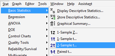
- Step 1
Under the Stat menu, select Basic Statistics, and then select 2-Sample t...:
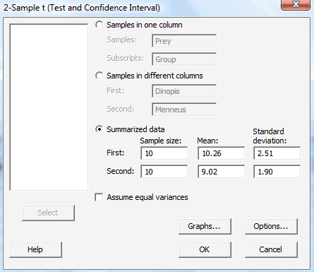
- Step 2
In the pop-up window that appears, select Summarized data. Then, for the First variable (deinopis data, for us), type the Sample size, Mean, and Standard deviation in the appropriate boxes. Do the same thing for the Second variable (menneus data, for us), that is, type the Sample size, Mean, and Standard deviation in the appropriate boxes. Select Ok:
The confidence interval output will appear in the session window. Here's what the output looks like for the spider and prey example with the confidence interval circled in red:
Two-Sample T-Test and CI
| Sample | N | Mean | StDev | SE Mean |
|---|---|---|---|---|
| 1 | 10 | 10.26 | 2.51 | 0.79 |
| 2 | 10 | 9.02 | 1.90 | 0.60 |
Difference = mu (1) - mu (2)
Estimate for difference: 1.240
95% CI for difference: (-0.870, 3.350)
T-Test of difference = 0 (vs not =): T-Value = 1.25 P-Value = 0.231 DF = 16