Lesson 4: Confidence Intervals for Variances
Lesson 4: Confidence Intervals for VariancesHey, we've checked off the estimation of a number of population parameters already. Let's check off a few more! In this lesson, we'll derive \((1−\alpha)100\%\) confidence intervals for:
- a single population variance: \(\sigma^2\)
- the ratio of two population variances: \(\dfrac{\sigma^2_X}{\sigma^2_Y}\) or \(\dfrac{\sigma^2_Y}{\sigma^2_X}\)
Along the way, we'll take a side path to explore the characteristics of the probability distribution known as the F-distribution.
4.1 - One Variance
4.1 - One VarianceLet's start right out by stating the confidence interval for one population variance.
If \(X_{1}, X_{2}, \dots , X_{n}\) are normally distributed and \(a=\chi^2_{1-\alpha/2,n-1}\) and \(b=\chi^2_{\alpha/2,n-1}\), then a \((1−\alpha)\%\) confidence interval for the population variance \(\sigma^2\) is:
\(\left(\dfrac{(n-1)s^2}{b} \leq \sigma^2 \leq \dfrac{(n-1)s^2}{a}\right)\)
And a \((1−\alpha)\%\) confidence interval for the population standard deviation \(\sigma\) is:
\(\left(\dfrac{\sqrt{(n-1)}}{\sqrt{b}}s \leq \sigma \leq \dfrac{\sqrt{(n-1)}}{\sqrt{a}}s\right)\)
Proof
We learned previously that if \(X_{1}, X_{2}, \dots , X_{n}\) are normally distributed with mean \(\mu\) and population variance \(\sigma^2\), then:
\(\dfrac{(n-1)S^2}{\sigma^2} \sim \chi^2_{n-1}\)
Then, using the following picture as a guide:
with (\(a=\chi^2_{1-\alpha/2}\)) and (\(b=\chi^2_{\alpha/2}\)), we can write the following probability statement:
\(P\left[a\leq \dfrac{(n-1)S^2}{\sigma^2} \leq b\right]=1-\alpha\)
Now, as always it's just a matter of manipulating the quantity in the parentheses. That is:
\(a\leq \dfrac{(n-1)S^2}{\sigma^2} \leq b\)
Taking the reciprocal of all three terms, and thereby changing the direction of the inequalities, we get:
\(\dfrac{1}{a}\geq \dfrac{\sigma^2}{(n-1)S^2} \geq \dfrac{1}{b}\)
Now, multiplying through by \((n−1)S^2\), and rearranging the direction of the inequalities, we get the confidence interval for \(\sigma ^2\):
\(\dfrac{(n-1)S^2}{b} \leq \sigma^2 \leq \dfrac{(n-1)S^2}{a}\)
as was to be proved. And, taking the square root, we get the confidence interval for \(\sigma\):
\(\dfrac{\sqrt{(n-1)S^2}}{\sqrt{b}} \leq \sigma \leq \dfrac{\sqrt{(n-1)S^2}}{\sqrt{a}}\)
as was to be proved.
Example 32-1

A large candy manufacturer produces, packages and sells packs of candy targeted to weigh 52 grams. A quality control manager working for the company was concerned that the variation in the actual weights of the targeted 52-gram packs was larger than acceptable. That is, he was concerned that some packs weighed significantly less than 52-grams and some weighed significantly more than 52 grams. In an attempt to estimate \(\sigma\), the standard deviation of the weights of all of the 52-gram packs the manufacturer makes, he took a random sample of n = 10 packs off of the factory line. The random sample yielded a sample variance of 4.2 grams. Use the random sample to derive a 95% confidence interval for \(\sigma\).
Answer
First, we need to determine the two chi-square values with (n−1) = 9 degrees of freedom. Using the table in the back of the textbook, we see that they are:
\(a=\chi^2_{1-\alpha/2,n-1}=\chi^2_{0.975,9}=2.7\) and \(b=\chi^2_{\alpha/2,n-1}=\chi^2_{0.025,9}=19.02\)
Now, it's just a matter of substituting in what we know into the formula for the confidence interval for the population variance. Doing so, we get:
\(\left(\dfrac{9(4.2)}{19.02} \leq \sigma^2 \leq \dfrac{9(4.2)}{2.7}\right)\)
Simplifying, we get:
\((1.99\leq \sigma^2 \leq 14.0)\)
We can be 95% confident that the variance of the weights of all of the packs of candy coming off of the factory line is between 1.99 and 14.0 grams-squared. Taking the square root of the confidence limits, we get the 95% confidence interval for the population standard deviation \(\sigma\):
\((1.41\leq \sigma \leq 3.74)\)
That is, we can be 95% confident that the standard deviation of the weights of all of the packs of candy coming off of the factory line is between 1.41 and 3.74 grams.
Minitab®
Using Minitab
Confidence Interval for One Variance
-
Under the Stat menu, select Basic Statistics, and then select 1 Variance...:
-
In the pop-up window that appears, in the box labeled Data, select Sample variance. Then, fill in the boxes labeled Sample size and Sample variance.

-
Click on the button labeled Options... In the pop-up window that appears, specify the confidence level and "not equal" for the alternative.
Then, click on OK to return to the main pop-up window.
-
Then, upon clicking OK on the main pop-up window, the output should appear in the Session window:
Test and CI for One Variance
Method
The chi-square method is only for the normal distribution.
The Bonett method cannot be calculated with summarized data.
Statistics
| N | StDev | Variance |
|---|---|---|
| 10 | 2.05 | 4.20 |
95% Confidence Intervals
| Method | CI for StDev |
CI for Variance |
|---|---|---|
| Chi-Square | (1.41, 3.74) | (1.99, 14.00) |
4.2 - The F-Distribution
4.2 - The F-DistributionAs we'll soon see, the confidence interval for the ratio of two variances requires the use of the probability distribution known as the F-distribution. So, let's spend a few minutes learning the definition and characteristics of the F-distribution.
F-distribution
If U and V are independent chi-square random variables with \(r_1\) and \(r_2\) degrees of freedom, respectively, then:
\(F=\dfrac{U/r_1}{V/r_2}\)
follows an F-distribution with \(r_1\) numerator degrees of freedom and \(r_2\) denominator degrees of freedom. We write F ~ F(\(r_1\), \(r_2\)).
Characteristics of the F-Distribution
F-distributions are generally skewed. The shape of an F-distribution depends on the values of \(r_1\) and \(r_2\), the numerator and denominator degrees of freedom, respectively, as this picture pirated from your textbook illustrates:

The probability density function of an F random variable with \(r_1\) numerator degrees of freedom and \(r_2\) denominator degrees of freedom is:
\(f(w)=\dfrac{(r_1/r_2)^{r_1/2}\Gamma[(r_1+r_2)/2]w^{(r_1/2)-1}}{\Gamma[r_1/2]\Gamma[r_2/2][1+(r_1w/r_2)]^{(r_1+r_2)/2}}\)
over the support \(w ≥ 0\).
The definition of an F-random variable:
\(F=\dfrac{U/r_1}{V/r_2}\)
implies that if the distribution of W is F(\(r_1\), \(r_2\)), then the distribution of 1/W is F(\(r_2\), \(r_1\)).
The F-Table
One of the primary ways that we will need to interact with an F-distribution is by needing to know either:
- An F-value, or
- The probabilities associated with an F-random variable, in order to complete a statistical analysis.
We could go ahead and try to work with the above probability density function to find the necessary values, but I think you'll agree before long that we should just turn to an F-table, and let it do the dirty work for us. For that reason, we'll now explore how to use a typical F-table to look up F-values and/or F-probabilities. Let's start with two definitions.
\(100 \alpha^{th}\) percentile
Let \(\alpha\) be some probability between 0 and 1 (most often, a small probability less than 0.10). The upper \(100 \alpha^{th}\) percentile of an F-distribution with \(r_1\) and \(r_2\) degrees of freedom is the value \(F_\alpha(r_1,r_2)\) such that the area under the curve and to the right of \(F_\alpha(r_1,r_2)\) is \(\alpha\):
The above definition is used in Table VII, the F-distribution table in the back of your textbook. While the next definition is not used directly in Table VII, you'll still find it necessary when looking for F-values (or F-probabilities) in the left tail of an F-distribution.
\(100 \alpha^{th}\) percentile
Let \(\alpha\) be some probability between 0 and 1 (most often, a small probability less than 0.10). The \(100 \alpha^{th}\) percentile of an F-distribution with \(r_1\) and \(r_2\) degrees of freedom is the value \(F_{1-\alpha}(r_1,r_2)\) such that the area under the curve and to the right of \(F_{1-\alpha}(r_1,r_2)\) is 1−\(\alpha\):

With the two definitions behind us, let's now take a look at the F-table in the back of your textbook.
In summary, here are the steps you should take in using the F>-table to find an F-value:
- Find the column that corresponds to the relevant numerator degrees of freedom, \(r_1\).
- Find the three rows that correspond to the relevant denominator degrees of freedom, \(r_2\).
- Find the one row, from the group of three rows identified in the second step, that is headed by the probability of interest... whether it's 0.01, 0.025, 0.05.
- Determine the F-value where the \(r_1\) column and the probability row identified in step 3 intersect.
Now, at least theoretically, you could also use the F-table to find the probability associated with a particular F-value. But, as you can see, the table is pretty (very!) limited in that direction. For example, if you have an F random variable with 6 numerator degrees of freedom and 2 denominator degrees of freedom, you could only find the probabilities associated with the F values of 19.33, 39.33, and 99.33:
\(P(F ≤ f)\) = \(\displaystyle \int^f_0\dfrac{\Gamma[(r_1+r_2)/2](r_1/r_2)^{r_1/2}w^{(r_1/2)-1}}{\Gamma[r_1/2]\Gamma[r_2/2][1+(r_1w/r_2)]^{(r_1+r_2)/2}}dw\) | ||||||||||
|---|---|---|---|---|---|---|---|---|---|---|
\(\alpha\) | \(P(F ≤ f)\) | Den. | Numerator Degrees of Freedom, \(r_1\) | |||||||
1 | 2 | 3 | 4 | 5 | 6 | 7 | 8 | |||
0.05 | 0.95 | 1 | 161.40 | 199.50 | 215.70 | 224.60 | 230.20 | 234.00 | 236.80 | 238.90 |
0.05 | 0.95 | 2 | 18.51 | 19.00 | 19.16 | 19.25 | 19.30 | 19.33 | 19.35 | 19.37 |
What would you do if you wanted to find the probability that an F random variable with 6 numerator degrees of freedom and 2 denominator degrees of freedom was less than 6.2, say? Well, the answer is, of course... statistical software, such as SAS or Minitab! For what we'll be doing, the F table will (mostly) serve our purpose. When it doesn't, we'll use Minitab. At any rate, let's get a bit more practice now using the F table.
Example 4-2
Let X be an F random variable with 4 numerator degrees of freedom and 5 denominator degrees of freedom. What is the upper fifth percentile?
Answer
The upper fifth percentile is the F-value x such that the probability to the right of x is 0.05, and therefore the probability to the left of x is 0.95. To find x using the F-table, we:
- Find the column headed by \(r_1 = 4\).
- Find the three rows that correspond to \(r_2 = 5\).
- Find the one row, from the group of three rows identified in the above step, that is headed by \(\alpha = 0.05\) (and \(P(X ≤ x) = 0.95\).
Now, all we need to do is read the F-value where the \(r_1 = 4\) column and the identified \(\alpha = 0.05\) row intersect. What do you get?
\(P(F ≤ f)\) = \(\displaystyle \int^f_0\dfrac{\Gamma[(r_1+r_2)/2](r_1/r_2)^{r_1/2}w^{(r_1/2)-1}}{\Gamma[r_1/2]\Gamma[r_2/2][1+(r_1w/r_2)]^{(r_1+r_2)/2}}dw\) | ||||||||||
|---|---|---|---|---|---|---|---|---|---|---|
\(\alpha\) | \(P(F ≤ f)\) | Den. | Numerator Degrees of Freedom, \(r_1\) | |||||||
1 | 2 | 3 | 4 | 5 | 6 | 7 | 8 | |||
0.05 | 0.95 | 1 | 161.40 | 199.50 | 215.70 | 224.60 | 230.20 | 234.00 | 236.80 | 238.90 |
0.05 | 0.95 | 2 | 18.51 | 19.00 | 19.16 | 19.25 | 19.30 | 19.33 | 19.35 | 19.37 |
0.05 | 0.95 | 3 | 10.13 | 9.55 | 9.28 | 9.12 | 9.01 | 8.94 | 8.89 | 8.85 |
0.05 | 0.95 | 4 | 7.71 | 6.94 | 6.59 | 6.39 | 6.26 | 6.16 | 6.09 | 6.04 |
0.05 | 0.95 | 5 | 6.61 | 5.79 | 5.41 | 5.19 | 5.05 | 4.95 | 4.88 | 4.82 |
0.05 | 0.95 | 6 | 5.99 | 5.14 | 4.76 | 4.53 | 4.39 | 4.28 | 4.21 | 4.15 |
The table tells us that the upper fifth percentile of an F random variable with 4 numerator degrees of freedom and 5 denominator degrees of freedom is 5.19.
Let X be an F random variable with 4 numerator degrees of freedom and 5 denominator degrees of freedom. What is the first percentile?
Answer
The first percentile is the F-value x such that the probability to the left of x is 0.01 (and hence the probability to the right of x is 0.99). Since such an F-value isn't directly readable from the F-table, we need to do a little finagling to find x using the F-table. That is, we need to recognize that the F-value we are looking for, namely \(F_{0.99}(4,5)\), is related to \(F_{0.01}(5,4)\), a value we can read off of the table by way of this relationship:
\(F_{0.99}(4,5)=\dfrac{1}{F_{0.01}(5,4)}\)
That said, to find x using the F-table, we:
- Find the column headed by \(r_1 = 5\).
- Find the three rows that correspond to \(r_2 = 4\).
- Find the one row, from the group of three rows identified in (2), that is headed by \(\alpha = 0.01\) (and \(P(X ≤ x) = 0.99\).
Now, all we need to do is read the F-value where the \(r_1 = 5\) column and the identified \(\alpha = 0.01\) row intersect, and take the inverse. What do you get?
\(P(F ≤ f)\) = \(\displaystyle \int^f_0\dfrac{\Gamma[(r_1+r_2)/2](r_1/r_2)^{r_1/2}w^{(r_1/2)-1}}{\Gamma[r_1/2]\Gamma[r_2/2][1+(r_1w/r_2)]^{(r_1+r_2)/2}}dw\) | ||||||||||
|---|---|---|---|---|---|---|---|---|---|---|
\(\alpha\) | \(P(F ≤ f)\) | Den. | Numerator Degrees of Freedom, \(r_1\) | |||||||
1 | 2 | 3 | 4 | 5 | 6 | 7 | 8 | |||
0.05 | 0.95 | 1 | 161.40 | 199.50 | 215.70 | 224.60 | 230.20 | 234.00 | 236.80 | 238.90 |
0.05 | 0.95 | 2 | 18.51 | 19.00 | 19.16 | 19.25 | 19.30 | 19.33 | 19.35 | 19.37 |
0.05 | 0.95 | 3 | 10.13 | 9.55 | 9.28 | 9.12 | 9.01 | 8.94 | 8.89 | 8.85 |
0.05 | 0.95 | 4 | 7.71 | 6.94 | 6.59 | 6.39 | 6.26 | 6.16 | 6.09 | 6.04 |
0.05 | 0.95 | 5 | 6.61 | 5.79 | 5.41 | 5.19 | 5.05 | 4.95 | 4.88 | 4.82 |
0.05 | 0.95 | 6 | 5.99 | 5.14 | 4.76 | 4.53 | 4.39 | 4.28 | 4.21 | 4.15 |
The table, along with a minor calculation, tells us that the first percentile of an F random variable with 4 numerator degrees of freedom and 5 denominator degrees of freedom is 1/15.52 = 0.064.
What is the probability that an F random variable with 4 numerator degrees of freedom and 5 denominator degrees of freedom is greater than 7.39?
Answer
There I go... just a minute ago, I said that the F-table isn't very helpful in finding probabilities, then I turn around and ask you to use the table to find a probability! Doing it at least once helps us make sure that we fully understand the table. In this case, we are going to need to read the table "backwards." To find the probability, we:
- Find the column headed by \(r_1 = 4\).
- Find the three rows that correspond to \(r_2 = 5\).
- Find the one row, from the group of three rows identified in the second point above, that contains the value 7.39 in the \(r_1 = 4\) column.
- Read the value of \(\alpha\) that heads the row in which the 7.39 falls.
What do you get?
\(P(F ≤ f)\) = \(\displaystyle \int^f_0\dfrac{\Gamma[(r_1+r_2)/2](r_1/r_2)^{r_1/2}w^{(r_1/2)-1}}{\Gamma[r_1/2]\Gamma[r_2/2][1+(r_1w/r_2)]^{(r_1+r_2)/2}}dw\) | ||||||||||
|---|---|---|---|---|---|---|---|---|---|---|
\(\alpha\) | \(P(F ≤ f)\) | Den. | Numerator Degrees of Freedom, \(r_1\) | |||||||
1 | 2 | 3 | 4 | 5 | 6 | 7 | 8 | |||
0.05 | 0.95 | 1 | 161.40 | 199.50 | 215.70 | 224.60 | 230.20 | 234.00 | 236.80 | 238.90 |
0.05 | 0.95 | 2 | 18.51 | 19.00 | 19.16 | 19.25 | 19.30 | 19.33 | 19.35 | 19.37 |
0.05 | 0.95 | 3 | 10.13 | 9.55 | 9.28 | 9.12 | 9.01 | 8.94 | 8.89 | 8.85 |
0.05 | 0.95 | 4 | 7.71 | 6.94 | 6.59 | 6.39 | 6.26 | 6.16 | 6.09 | 6.04 |
0.05 | 0.95 | 5 | 6.61 | 5.79 | 5.41 | 5.19 | 5.05 | 4.95 | 4.88 | 4.82 |
0.05 | 0.95 | 6 | 5.99 | 5.14 | 4.76 | 4.53 | 4.39 | 4.28 | 4.21 | 4.15 |
The table tells us that the probability that an F random variable with 4 numerator degrees of freedom and 5 denominator degrees of freedom is greater than 7.39 is 0.025.
4.3 - Two Variances
4.3 - Two VariancesNow that we have the characteristics of the F-distribution behind us, let's again jump right in by stating the confidence interval for the ratio of two population variances.
If \(X_1,X_2,\ldots,X_n \sim N(\mu_X,\sigma^2_X)\) and \(Y_1,Y_2,\ldots,Y_m \sim N(\mu_Y,\sigma^2_Y)\) are independent random samples, and:
-
\(c=F_{1-\alpha/2}(m-1,n-1)=\dfrac{1}{F_{\alpha/2}(n-1,m-1)}\) and
-
\(d=F_{\alpha/2}(m-1,n-1)\),
then a \((1−\alpha) 100\%\) confidence interval for \(\sigma^2_X/\sigma^2_Y\) is:
\(\left(\dfrac{1}{F_{\alpha/2}(n-1,m-1)} \dfrac{s^2_X}{s^2_Y} \leq \dfrac{\sigma^2_X}{\sigma^2_Y}\leq F_{\alpha/2}(m-1,n-1)\dfrac{s^2_X}{s^2_Y}\right)\)
Proof
Because \(X_1,X_2,\ldots,X_n \sim N(\mu_X,\sigma^2_X)\) and \(Y_1,Y_2,\ldots,Y_m \sim N(\mu_Y,\sigma^2_Y)\) , it tells us that:
\(\dfrac{(n-1)S^2_X}{\sigma^2_X}\sim \chi^2_{n-1}\) and \(\dfrac{(m-1)S^2_Y}{\sigma^2_Y}\sim \chi^2_{m-1}\)
Then, by the independence of the two samples, we well as the definition of an F random variable, we know that:
\(F=\dfrac{\dfrac{(m-1)S^2_Y}{\sigma^2_Y}/(m-1)}{\dfrac{(n-1)S^2_X}{\sigma^2_X}/(n-1)}=\dfrac{\sigma^2_X}{\sigma^2_Y}\cdot \dfrac{S^2_Y}{S^2_X} \sim F(m-1,n-1)\)
Therefore, the following probability statement holds:
\(P\left[F_{1-\frac{\alpha}{2}}(m-1,n-1) \leq \dfrac{\sigma^2_X}{\sigma^2_Y}\cdot \dfrac{S^2_Y}{S^2_X} \leq F_{\frac{\alpha}{2}}(m-1,n-1)\right]=1-\alpha\)
Finding the \((1-\alpha)100\%\) confidence interval for the ratio of the two population variances then reduces, as always, to manipulating the quantity in parentheses. Multiplying through the inequality by:
\(\dfrac{S^2_X}{S^2_Y}\)
and recalling the fact that:
\(F_{1-\frac{\alpha}{2}}(m-1,n-1)=\dfrac{1}{F_{\frac{\alpha}{2}}(n-1,m-1)}\)
the \((1-\alpha)100\%\) confidence interval for the ratio of the two population variances reduces to:
\(\dfrac{1}{F_{\frac{\alpha}{2}}(n-1,m-1)}\dfrac{S^2_X}{S^2_Y}\leq \dfrac{\sigma^2_X}{\sigma^2_Y} \leq F_{\frac{\alpha}{2}}(m-1,n-1)\dfrac{S^2_X}{S^2_Y}\)
as was to be proved.
Example 4-3
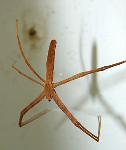
Let's return to the example, in which the feeding habits of two-species of net-casting spiders are studied. The species, the deinopis and menneus, coexist in eastern Australia. The following summary statistics were obtained on the size, in millimeters, of the prey of the two species:
| Adult DEINOPIS | Adult MENNEUS |
|---|---|
| \(n\) = 10 | \(m\) = 10 |
| \(\bar{x}\) = 10.26 mm | \(\bar{y}\) = 9.02 mm |
| \({s^2_X}\)= \((2.51)^2\) | \({s^2_Y}\) = \((1.90)^2\) |
Estimate, with 95% confidence, the ratio of the two population variances.
Answer
In order to estimate the ratio of the two population variances, we need to obtain two F-values from the F-table, namely:
\(F_{0.025}(9,9)=4.03\) and \(F_{0.975}(9,9)=\dfrac{1}{F_{0.025}(9,9)}=\dfrac{1}{4.03}\)
Then, the 95% confidence interval for the ratio of the two population variances is:
\(\dfrac{1}{4.03} \left(\dfrac{2.51^2}{1.90^2}\right) \leq \dfrac{\sigma^2_X}{\sigma^2_Y} \leq 4.03 \left(\dfrac{2.51^2}{1.90^2}\right)\)
Simplifying, we get:
\(0.433\leq \dfrac{\sigma^2_X}{\sigma^2_Y} \leq7.033\)
That is, we can be 95% confident that the ratio of the two population variances is between 0.433 and 7.033. (Because the interval contains the value 1, we cannot conclude that the population variances differ.)
Now that we've spent two pages learning confidence intervals for variances, I have a confession to make. It turns out that confidence intervals for variances have generally lost favor with statisticians, because they are not very accurate when the data are not normally distributed. In that case, we say they are "sensitive" to the normality assumption, or the intervals are "not robust."
Minitab®
Using Minitab
Confidence Interval for Two Variances
-
Under the Stat menu, select Basic Statistics, and then select 2 Variances...:
-
In the pop-up window that appears, in the box labeled Data, select Sample standard deviations (or alternatively Sample variances). In the box labeled Sample size, type in the size n of the First sample and m of the Second sample. In the box labeled Standard deviation, type in the sample standard deviations for the First and Second samples:

-
Click on the button labeled Options... In the pop-up window that appears, specify the confidence level, and in the box labeled Alternative, select not equal.
Then, click on OK to return to the main pop-up window.
-
Then, upon clicking OK on the main pop-up window, the output should appear in the Session window:
Test and CI for Two Variances
Method
Null hypothesis Sigma (1) / Sigma (2) = 1
Alternative hypothesis Sigma (1) / Sigma (2) not = 1
Significance level Alpha = 0.05
Statistics
| Sample | N | StDev | Variance |
|---|---|---|---|
| 1 | 10 | 2.510 | 6.300 |
| 2 | 10 | 1.900 | 3.610 |
Ratio of standard deviations = 1.321
Ratio of variances = 1.745
95% Confidence Intervals
| Distribution of Data |
CI for StDev Ratio |
CI for Variance Ratio |
|---|---|---|
| Normal | (0.685, 2.651) | (0.433, 7.026) |