4.3 - Two Variances
4.3 - Two VariancesNow that we have the characteristics of the F-distribution behind us, let's again jump right in by stating the confidence interval for the ratio of two population variances.
If \(X_1,X_2,\ldots,X_n \sim N(\mu_X,\sigma^2_X)\) and \(Y_1,Y_2,\ldots,Y_m \sim N(\mu_Y,\sigma^2_Y)\) are independent random samples, and:
-
\(c=F_{1-\alpha/2}(m-1,n-1)=\dfrac{1}{F_{\alpha/2}(n-1,m-1)}\) and
-
\(d=F_{\alpha/2}(m-1,n-1)\),
then a \((1−\alpha) 100\%\) confidence interval for \(\sigma^2_X/\sigma^2_Y\) is:
\(\left(\dfrac{1}{F_{\alpha/2}(n-1,m-1)} \dfrac{s^2_X}{s^2_Y} \leq \dfrac{\sigma^2_X}{\sigma^2_Y}\leq F_{\alpha/2}(m-1,n-1)\dfrac{s^2_X}{s^2_Y}\right)\)
Proof
Because \(X_1,X_2,\ldots,X_n \sim N(\mu_X,\sigma^2_X)\) and \(Y_1,Y_2,\ldots,Y_m \sim N(\mu_Y,\sigma^2_Y)\) , it tells us that:
\(\dfrac{(n-1)S^2_X}{\sigma^2_X}\sim \chi^2_{n-1}\) and \(\dfrac{(m-1)S^2_Y}{\sigma^2_Y}\sim \chi^2_{m-1}\)
Then, by the independence of the two samples, we well as the definition of an F random variable, we know that:
\(F=\dfrac{\dfrac{(m-1)S^2_Y}{\sigma^2_Y}/(m-1)}{\dfrac{(n-1)S^2_X}{\sigma^2_X}/(n-1)}=\dfrac{\sigma^2_X}{\sigma^2_Y}\cdot \dfrac{S^2_Y}{S^2_X} \sim F(m-1,n-1)\)
Therefore, the following probability statement holds:
\(P\left[F_{1-\frac{\alpha}{2}}(m-1,n-1) \leq \dfrac{\sigma^2_X}{\sigma^2_Y}\cdot \dfrac{S^2_Y}{S^2_X} \leq F_{\frac{\alpha}{2}}(m-1,n-1)\right]=1-\alpha\)
Finding the \((1-\alpha)100\%\) confidence interval for the ratio of the two population variances then reduces, as always, to manipulating the quantity in parentheses. Multiplying through the inequality by:
\(\dfrac{S^2_X}{S^2_Y}\)
and recalling the fact that:
\(F_{1-\frac{\alpha}{2}}(m-1,n-1)=\dfrac{1}{F_{\frac{\alpha}{2}}(n-1,m-1)}\)
the \((1-\alpha)100\%\) confidence interval for the ratio of the two population variances reduces to:
\(\dfrac{1}{F_{\frac{\alpha}{2}}(n-1,m-1)}\dfrac{S^2_X}{S^2_Y}\leq \dfrac{\sigma^2_X}{\sigma^2_Y} \leq F_{\frac{\alpha}{2}}(m-1,n-1)\dfrac{S^2_X}{S^2_Y}\)
as was to be proved.
Example 4-3
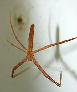
Let's return to the example, in which the feeding habits of two-species of net-casting spiders are studied. The species, the deinopis and menneus, coexist in eastern Australia. The following summary statistics were obtained on the size, in millimeters, of the prey of the two species:
| Adult DEINOPIS | Adult MENNEUS |
|---|---|
| \(n\) = 10 | \(m\) = 10 |
| \(\bar{x}\) = 10.26 mm | \(\bar{y}\) = 9.02 mm |
| \({s^2_X}\)= \((2.51)^2\) | \({s^2_Y}\) = \((1.90)^2\) |
Estimate, with 95% confidence, the ratio of the two population variances.
Answer
In order to estimate the ratio of the two population variances, we need to obtain two F-values from the F-table, namely:
\(F_{0.025}(9,9)=4.03\) and \(F_{0.975}(9,9)=\dfrac{1}{F_{0.025}(9,9)}=\dfrac{1}{4.03}\)
Then, the 95% confidence interval for the ratio of the two population variances is:
\(\dfrac{1}{4.03} \left(\dfrac{2.51^2}{1.90^2}\right) \leq \dfrac{\sigma^2_X}{\sigma^2_Y} \leq 4.03 \left(\dfrac{2.51^2}{1.90^2}\right)\)
Simplifying, we get:
\(0.433\leq \dfrac{\sigma^2_X}{\sigma^2_Y} \leq7.033\)
That is, we can be 95% confident that the ratio of the two population variances is between 0.433 and 7.033. (Because the interval contains the value 1, we cannot conclude that the population variances differ.)
Now that we've spent two pages learning confidence intervals for variances, I have a confession to make. It turns out that confidence intervals for variances have generally lost favor with statisticians, because they are not very accurate when the data are not normally distributed. In that case, we say they are "sensitive" to the normality assumption, or the intervals are "not robust."
Minitab®
Using Minitab
Confidence Interval for Two Variances
-
Under the Stat menu, select Basic Statistics, and then select 2 Variances...:
-
In the pop-up window that appears, in the box labeled Data, select Sample standard deviations (or alternatively Sample variances). In the box labeled Sample size, type in the size n of the First sample and m of the Second sample. In the box labeled Standard deviation, type in the sample standard deviations for the First and Second samples:

-
Click on the button labeled Options... In the pop-up window that appears, specify the confidence level, and in the box labeled Alternative, select not equal.
Then, click on OK to return to the main pop-up window.
-
Then, upon clicking OK on the main pop-up window, the output should appear in the Session window:
Test and CI for Two Variances
Method
Null hypothesis Sigma (1) / Sigma (2) = 1
Alternative hypothesis Sigma (1) / Sigma (2) not = 1
Significance level Alpha = 0.05
Statistics
| Sample | N | StDev | Variance |
|---|---|---|---|
| 1 | 10 | 2.510 | 6.300 |
| 2 | 10 | 1.900 | 3.610 |
Ratio of standard deviations = 1.321
Ratio of variances = 1.745
95% Confidence Intervals
| Distribution of Data |
CI for StDev Ratio |
CI for Variance Ratio |
|---|---|---|
| Normal | (0.685, 2.651) | (0.433, 7.026) |