5.1 - One Proportion
5.1 - One ProportionExample 5-1
The article titled "Poll shows increasing concern, little impact with malpractice crisis" in the February 20th, 2003 issue of the Centre Daily Times reported that \(n=418\) Pennsylvanians were surveyed about their opinions about insurance rates. Of the 418 surveyed, \(Y=280\) blamed rising insurance rates on large court settlements against doctors. That is, the sample proportion is:
\(\hat{p}=\dfrac{280}{418}=0.67\)
Use this sample proportion to estimate, with 95% confidence, the parameter \(p\), that is, the proportion of all Pennsylvanians who blame rising insurance rates on large court settlements against doctors.
Answer
We'll need some theory before we can really find the confidence interval for the population proportion \(p\), but we can at least get the ball rolling here. Let:
- \(X_i=1\), if randomly selected Pennsylvanian \(i\) blames rising insurance rates on large court settlements against doctors
- \(X_i=0\), if randomly selected Pennsylvanian \(i\) does not blame rising insurance rates on large court settlements against doctors
Then, the number of Pennsylvanians in the random sample who blame rising insurance rates on large court settlements against doctors is:
\(Y=\sum\limits_{i=1}^{418} X_i=280\)
and therefore, the proportion of Pennsylvanians in the random sample who blame rising insurance rates on large court settlements against doctors is:
\(\hat{p}=\dfrac{\sum_{i=1}^n X_i}{n}=\dfrac{280}{418}=0.67\)
Well, alright, so we're right back where we started, as we basically just repeated what we were given. Well, not quite! That most recent sample proportion was written in order to emphasize the fact that a sample proportion can really be thought of as just a sample average (of 0 and 1 data):
\(\hat{p}=\frac{\sum_{i=1}^n X_i }{n}=0.67\)
Ohhhhh... so that means we can use what we know about the sampling distribution of \(\bar{X}\) to derive a confidence interval for the population proportion \(p\).
Let's jump ahead and state the result, and then we'll step back and prove it.
Theorem
For large random samples, a \((1-\alpha)100\%\) confidence interval for a population proportion \(p\) is:
\(\hat{p}-z_{\alpha/2}\sqrt{\dfrac{\hat{p}(1-\hat{p})}{n}} \leq p \leq \hat{p}+z_{\alpha/2}\sqrt{\dfrac{\hat{p}(1-\hat{p})}{n}}\)
Proof
Okay, so where were we? That's right... we were talking about the the sampling distribution of \(\bar{X}\). Well, we know that the Central Limit Theorem tells us, for large \(n\), that:
\(Z=\dfrac{\bar{X}-\mu}{\sigma/\sqrt{n}}\)
follows, at least approximately, a standard normal distribution \(N(0,1)\). Now, because:
\(Z=\dfrac{\bar{x}-\mu}{\sigma/\sqrt{n}}, \qquad \bar{x}=\hat{p}, \qquad \mu=E(X_i)=p, \qquad \sigma^2=\text{Var}(X_i)=p(1-p) \Rightarrow Z=\frac{\hat{p}-p}{\sqrt{\frac{p(1-p)}{n}}}\)
that implies, for large \(n\), that:
\(Z=\dfrac{\hat{p}-p}{\sqrt{\dfrac{p(1-p)}{n}}}\)
also follows, at least approximately, a standard normal distribution \(N(0,1)\). So, we can do our usual trick of starting with a probability statement:
\(P \left[-z_{\alpha/2}\leq \dfrac{\hat{p}-p}{\sqrt{\dfrac{p(1-p)}{n}}} \leq z_{\alpha/2}\right] \approx 1-\alpha\)
and manipulating the quantity inside the parentheses:
\(-z_{\alpha/2}\leq \dfrac{\hat{p}-p}{\sqrt{\dfrac{p(1-p)}{n}}} \leq z_{\alpha/2} \)
to get the formula for a \((1-\alpha)100\%\) confidence interval for \(p\). Multiplying through the inequality by the quantity in the denominator, we get:
\(-z_{\alpha/2} \sqrt{\dfrac{p(1-p)}{n}} \leq \hat{p}-p \leq z_{\alpha/2} \sqrt{\dfrac{p(1-p)}{n}}\)
Subtracting through the inequality by \(\hat{p}\), we get:
\(-\hat{p}-z_{\alpha/2} \sqrt{\dfrac{p(1-p)}{n}} \leq -p \leq -\hat{p}+z_{\alpha/2}\sqrt{\dfrac{p(1-p)}{n}}\)
And, upon dividing through by −1, and thereby reversing the inequality, we get the claimed \((1-\alpha)100\%\) confidence interval for \(p\):
\(\hat{p}-z_{\alpha/2} \sqrt{\dfrac{p(1-p)}{n}} \leq p \leq \hat{p}+z_{\alpha/2} \sqrt{\dfrac{p(1-p)}{n}}\)
Oooops! What's wrong with that confidence interval? Hmmmm.... it appears that we need to know the population proportion \(p\) in order to estimate the population proportion \(p\).
That's clearly not going to work. What's the logical thing to do? That's right... replace the population proportions (\(p\)) that appear in the endpoints of the interval with sample proportions (\(\hat{p}\)) to get an (approximate) \((1-\alpha)100\%\) confidence interval for \(p\):
\(\hat{p}-z_{\alpha/2} \sqrt{\dfrac{\hat{p}(1-\hat{p})}{n}} \leq p \leq \hat{p}+z_{\alpha/2} \sqrt{\dfrac{\hat{p}(1-\hat{p})}{n}}\)
as was to be proved!
Now that we have that theory behind us, let's return to our example!
Example 5-1 (continued)
The article titled "Poll shows increasing concern, little impact with malpractice crisis" in the February 20th issue of the Centre Daily Times reported that \(n=418\) Pennsylvanians were surveyed about their opinions about insurance rates. Of the 418 surveyed, \(Y=280\) blamed rising insurance rates on large court settlements against doctors. That is, the sample proportion is:
\(\hat{p}=\dfrac{280}{418}=0.67\)
Use this sample proportion to estimate, with 95% confidence, the parameter \(p\), that is, the proportion of all Pennsylvanians who blame rising insurance rates on large court settlements against doctors.
Answer
Plugging \(n=418\), a sample proportion of 0.67, and \(z_{0.025}=1.96\) into the formula for a 95% confidence interval for \(p\), we get:
\(0.67 \pm 1.96\sqrt{\dfrac{0.67(1-0.67)}{418}}\)
which, upon simplifying, is:
\(0.67 \pm 0.045\)
which equals:
\((0.625,0.715)\)
We can be 95% confident that between 62.5% and 71.5% of all Pennsylvanians blame rising insurance rates on large court settlements against doctors.
Minitab®
Using Minitab
As is always the case, you will probably want to calculate your confidence intervals for proportions using statistical software, such as Minitab, rather than doing it by way of formula and calculator. It's easy enough to calculate the (approximate) confidence interval for \(p\) using Minitab:
-
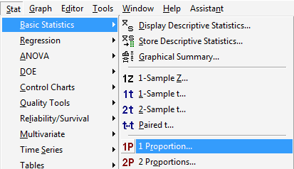
Under the Stat menu, select Basic Statistics, and then 1 Proportion...:

-
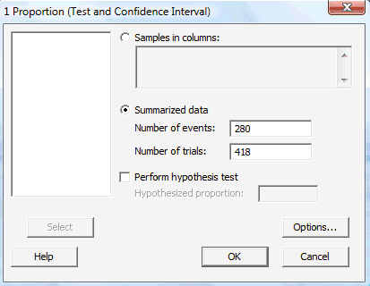
In the pop-up window that appears, select Summarized data, and enter the Number of events of interest that occurred, as well as the Number of trials (that is, the sample size n):

-
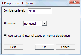
Click on the Options... button. If you want a confidence level that differs from the default 95.0 level, specify the desired level in the box labeled Confidence level. Click on the box labeled Use test and interval based on normal distribution. Select OK.

-
Select OK again on the primary pop-up window. The output should appear in the Session window:
Test and CI for One Proportion
| Sample | X | N | Sample p | 95% CI |
|---|---|---|---|---|
| 1 | 280 | 418 | 0.669856 | (0.624775, 0.714938) |
Using the normal approximation.
Notes
- Step 1
Our calculated margin of error is 4.5%:
\(0.67\pm \mathbf{0.045}\)
But, if you go back and take a look at the original article ("Poll shows increasing concern, little impact with malpractice crisis"), the newspaper's reported margin of error is 4.8%. What happened here? Why the difference? One possibility is that the newspaper was taking advantage of what is known about the maximum value of:
\(\hat{p}(1-\hat{p})\)
That is, the maximum value can be shown to be \(\frac{1}{4}\), as demonstrated here:
If we graph the function \(\hat{p}(1-\hat{p})\), it looks (roughly) like this:
We need to find the peak value, that is, the value marked by the red question mark (?). We can do that, of course, by taking the derivative of the function with respect to \(\hat{p}\), setting to 0, and solving for \(\hat{p}\). Taking the derivative and setting to 0, we get:
\(\dfrac{d(\hat{p}-\hat{p}^2)}{d\hat{p}}=1-2\hat{p}\equiv 0\)
And, solving for \(\hat{p}\), we get:
\(\hat{p}=\dfrac{1}{2}\)
Well, that's encouraging... the point at which we've determined that the maximum occurs at least agrees with our graph! Now, what is the value of the function \(\hat{p}(1-\hat{p})\) when \(\hat{p}=\dfrac{1}{2}\)? Well, it is:
\(\hat{p}-\hat{p}^2=\dfrac{1}{2}-\left(\dfrac{1}{2}\right)^2=\dfrac{1}{2}-\dfrac{1}{4}=\dfrac{1}{4}\)
as was claimed.
Because the maximum value of \(\hat{p}(1-\hat{p})\) can be shown to be \(\frac{1}{4}\), the largest the margin of error can be for a 95% confidence interval based on a sample size of \(n=418\) is:
\(1.96\sqrt{\dfrac{\frac{1}{2}(1-\frac{1}{2})}{418}} \approx 2\sqrt{\dfrac{1}{4}} \sqrt{\dfrac{1}{418}}=0.0489\)
Aha! First, that 95% margin of error looks eerily similar to the margin of error claimed by the newspaper. And second, that margin of error makes it look as if we can generalize a bit. Did you notice how we've reduced the 95% margin of error to an (approximate) function of the sample size \(n\)? In general, a 95% margin of error can be approximated by:
\(\dfrac{1}{\sqrt{n}}\)
Here's what that approximate 95% margin of error would like for various sample sizes \(n\):
-
\(n\) 25 64 100 900 1600 95% ME 0.20 0.125 0.10 0.033 0.025
By the way, it is of course entirely possible that the reported margin of error was not determined using the approximate 95% margin of error, as suggested above. It is feasible that the study's authors instead used a higher confidence level, or alternatively calculated the confidence interval using exact methods rather than the normal approximation. - Step 2
The approximate confidence interval for \(p\) that we derived above works well if the following two conditions hold simultaneously:
- \(np=\text{ the number of expected successes }\ge 5\)
- \(n(1-p)=\text{ the number of expected failures }\ge 5\)