9.1 - The Basic Idea

Every time we perform a hypothesis test, this is the basic procedure that we will follow:

We'll make an initial assumption about the population parameter.
We'll collect evidence or else use somebody else's evidence (in either case, our evidence will come in the form of data).
Based on the available evidence (data), we'll decide whether to "reject" or "not reject" our initial assumption.

Let's try to make this outlined procedure more concrete by taking a look at the following example.

Example 9-1

A four-sided (tetrahedral) die is tossed 1000 times, and 290 fours are observed. Is there evidence to conclude that the die is biased, that is, say, that more fours than expected are observed?

Answer

As the basic hypothesis testing procedure outlines above, the first step involves stating an initial assumption. It is:

Assume the die is unbiased. If the die is unbiased, then each side (1, 2, 3, and 4) is equally likely. So, we'll assume that p, the probability of getting a 4 is 0.25.

In general, the initial assumption is called the null hypothesis, and is denoted \(H_0\). (That's a zero in the subscript for "null"). In statistical notation, we write the initial assumption as:

\(H_0 \colon p=0.25\)

That is, the initial assumption involves making a statement about a population proportion.

Now, the second step tells us that we need to collect evidence (data) for or against our initial assumption. In this case, that's already been done for us. We were told that the die was tossed \(n=1000\) times, and \(y=290\) fours were observed. Using statistical notation again, we write the collected evidence as a sample proportion:

\(\hat{p}=\dfrac{y}{n}=\dfrac{290}{1000}=0.29\)

Now we just need to complete the third step of making the decision about whether or not to reject our initial assumption that the population proportion is 0.25. Recall that the Central Limit Theorem tells us that the sample proportion:

\(\hat{p}=\dfrac{Y}{n}\)

is approximately normally distributed with (assumed) mean:

\(p_0=0.25\)

and (assumed) standard deviation:

\(\sqrt{\dfrac{p_0(1-p_0)}{n}}=\sqrt{\dfrac{0.25(0.75)}{1000}}=0.01369\)

That means that:

\(Z=\dfrac{\hat{p}-p_0}{\sqrt{\dfrac{p_0(1-p_0)}{n}}}\)

follows a standard normal \(N(0,1)\) distribution. So, we can "translate" our observed sample proportion of 0.290 onto the \(Z\) scale. Here's a picture that summarizes the situation:

So, we are assuming that the population proportion is 0.25 (in blue), but we've observed a sample proportion 0.290 (in red) that falls way out in the right tail of the normal distribution. It certainly doesn't appear impossible to obtain a sample proportion of 0.29. But, that's what we're left with deciding. That is, we have to decide if a sample proportion of 0.290 is more extreme that we'd expect if the population proportion \(p\) does indeed equal 0.25.

There are two approaches to making the decision:

one is called the "critical value" (or "critical region" or "rejection region") approach
and the other is called the "\(p\)-value" approach

Until we get to the page in this lesson titled The \(p\)-value Approach, we'll use the critical value approach.

Example (continued)

A four-sided (tetrahedral) die is tossed 1000 times, and 290 fours are observed. Is there evidence to conclude that the die is biased, that is, say, that more fours than expected are observed?

Answer

Okay, so now let's think about it. We probably wouldn't reject our initial assumption that the population proportion \(p=0.25\) if our observed sample proportion were 0.255. And, we might still not be inclined to reject our initial assumption that the population proportion \(p=0.25\) if our observed sample proportion were 0.27. On the other hand, we would almost certainly want to reject our initial assumption that the population proportion \(p=0.25\) if our observed sample proportion were 0.35. That suggests, then, that there is some "threshold" value that once we "cross" the threshold value, we are inclined to reject our initial assumption. That is the critical value approach in a nutshell. That is, critical value approach tells us to define a threshold value, called a "critical value" so that if our "test statistic" is more extreme than the critical value, then we reject the null hypothesis.

Let's suppose that we decide to reject the null hypothesis \(H_0:p=0.25\) in favor of the "alternative hypothesis" \(H_A \colon p>0.25\) if:

\(\hat{p}>0.273\) or equivalently if \(Z>1.645\)

Here's a picture of such a "critical region" (or "rejection region"):

Note, by the way, that the "size" of the critical region is 0.05. This will become apparent in a bit when we talk below about the possible errors that we can make whenever we conduct a hypothesis test.

At any rate, let's get back to deciding whether our particular sample proportion appears to be too extreme. Well, it looks like we should reject the null hypothesis (our initial assumption \(p=0.25\)) because:

\(\hat{p}=0.29>0.273\)

or equivalently since our test statistic:

\(Z=\dfrac{\hat{p}-p_0}{\sqrt{\dfrac{p_0(1-p_0)}{n}}}=\dfrac{0.29-0.25}{\sqrt{\dfrac{0.25(0.75)}{1000}}}=2.92\)

is greater than 1.645.

Our conclusion: we say there is sufficient evidence to conclude \(H_A:p>0.25\), that is, that the die is biased.

By the way, this example involves what is called a one-tailed test, or more specifically, a right-tailed test, because the critical region falls in only one of the two tails of the normal distribution, namely the right tail.

Before we continue on the next page at looking at two more examples, let's revisit the basic hypothesis testing procedure that we outlined above. This time, though, let's state the procedure in terms of performing a hypothesis test for a population proportion using the critical value approach. The basic procedure is:

State the null hypothesis \(H_0\) and the alternative hypothesis \(H_A\). (By the way, some textbooks, including ours, use the notation \(H_1\) instead of \(H_A\) to denote the alternative hypothesis.)
Calculate the test statistic:
\(Z=\dfrac{\hat{p}-p_0}{\sqrt{\dfrac{p_0(1-p_0)}{n}}}\)
Determine the critical region.
Make a decision. Determine if the test statistic falls in the critical region. If it does, reject the null hypothesis. If it does not, do not reject the null hypothesis.

Now, back to those possible errors we can make when conducting such a hypothesis test.

Possible Errors

So, argh! Every time we conduct a hypothesis test, we have a chance of making an error. (Oh dear, why couldn't I have chosen a different profession?!)

If we reject the null hypothesis \(H_0\) (in favor of the alternative hypothesis \(H_A\)) when the null hypothesis is in fact true, we say we've committed a Type I error. For our example above, we set P(Type I error) equal to 0.05:
Aha! That's why the 0.05! We wanted to minimize our chance of making a Type I error! In general, we denote \(\alpha=P(\text{Type I error})=\) the "significance level of the test." Obviously, we want to minimize \(\alpha\). Therefore, typical \(\alpha\) values are 0.01, 0.05, and 0.10.
If we fail to reject the null hypothesis when the null hypothesis is false, we say we've committed a Type II error. For our example, suppose (unknown to us) that the population proportion \(p\) is actually 0.27. Then, the probability of a Type II error, in this case, is:
\(P(\text{Type II Error})=P(\hat{p}<0.273\quad if \quad p=0.27)=P\left(Z<\dfrac{0.273-0.27}{\sqrt{\dfrac{0.27(0.73)}{1000}}}\right)=P(Z<0.214)=0.5847\)
In general, we denote \(\beta=P(\text{Type II error})\). Just as we want to minimize \(\alpha=P(\text{Type I error})\), we want to minimize \(\beta=P(\text{Type II error})\). Typical \(\beta\) values are 0.05, 0.10, and 0.20.

9.2 - More Examples

Let's take a look at two more examples of a hypothesis test for a single proportion while recalling the hypothesis testing procedure we outlined on the previous page:

State the null hypothesis \(H_0\) and the alternative hypothesis \(H_{A}\).
Calculate the test statistic:

\(Z=\dfrac{\hat{p}-p_0}{\sqrt{\dfrac{p_0(1-p_0)}{n}}}\)
Determine the critical region.
Make a decision. Determine if the test statistic falls in the critical region. If it does, reject the null hypothesis. If it does not, do not reject the null hypothesis.

The first example involves a hypothesis test for the proportion in which the alternative hypothesis is a "greater than hypothesis," that is, the alternative hypothesis is of the form \(H_A \colon p > p_0\). And, the second example involves a hypothesis test for the proportion in which the alternative hypothesis is a "less than hypothesis," that is, the alternative hypothesis is of the form \(H_A \colon p < p_0\).

Example 9-2

Let p equal the proportion of drivers who use a seat belt in a state that does not have a mandatory seat belt law. It was claimed that \(p = 0.14\). An advertising campaign was conducted to increase this proportion. Two months after the campaign, \(y = 104\) out of a random sample of \(n = 590\) drivers were wearing seat belts. Was the campaign successful?

Answer

The observed sample proportion is:

\(\hat{p}=\dfrac{104}{590}=0.176\)

Because it is claimed that \(p = 0.14\), the null hypothesis is:

\(H_0 \colon p = 0.14\)

Because we're interested in seeing if the advertising campaign was successful, that is, that a greater proportion of people wear seat belts, the alternative hypothesis is:

\(H_A \colon p > 0.14\)

The test statistic is therefore:

\(Z=\dfrac{\hat{p}-p_0}{\sqrt{\dfrac{p_0(1-p_0)}{n}}}=\dfrac{0.176-0.14}{\sqrt{\dfrac{0.14(0.86)}{590}}}=2.52\)

If we use a significance level of \(\alpha = 0.01\), then the critical region is:

That is, we reject the null hypothesis if the test statistic \(Z > 2.326\). Because the test statistic falls in the critical region, that is, because \(Z = 2.52 > 2.326\), we can reject the null hypothesis in favor of the alternative hypothesis. There is sufficient evidence at the \(\alpha = 0.01\) level to conclude the campaign was successful (\(p > 0.14\)).

Again, note that this is an example of a right-tailed hypothesis test because the action falls in the right tail of the normal distribution.

Example 9-3

A Gallup poll released on October 13, 2000, found that 47% of the 1052 U.S. adults surveyed classified themselves as "very happy" when given the choices of:

"very happy"
"fairly happy"
"not too happy"

Suppose that a journalist who is a pessimist took advantage of this poll to write a headline titled "Poll finds that U.S. adults who are very happy are in the minority." Is the pessimistic journalist's headline warranted?

Answer

The sample proportion is:

\(\hat{p}=0.47\)

Because we're interested in the majority/minority boundary line, the null hypothesis is:

\(H_0 \colon p = 0.50\)

Because the journalist claims that the proportion of very happy U.S. adults is a minority, that is, less than 0.50, the alternative hypothesis is:

\(H_A \colon p < 0.50\)

The test statistic is therefore:

\(Z=\dfrac{\hat{p}-p_0}{\sqrt{\dfrac{p_0(1-p_0)}{n}}}=\dfrac{0.47-0.50}{\sqrt{\dfrac{0.50(0.50)}{1052}}}=-1.946\)

Now, this time, we need to put our critical region in the left tail of the normal distribution. If we use a significance level of \(\alpha = 0.05\), then the critical region is:

That is, we reject the null hypothesis if the test statistic \(Z < −1.645\). Because the test statistic falls in the critical region, that is, because \(Z = −1.946 < −1.645\), we can reject the null hypothesis in favor of the alternative hypothesis. There is sufficient evidence at the \(\alpha = 0.05\) level to conclude that \(p < 0.50\), that is, U.S. adults who are very happy are in the minority. The journalist's pessimism appears to be indeed warranted.

Note that this is an example of a left-tailed hypothesis test because the action falls in the left tail of the normal distribution.

9.3 - The P-Value Approach

Example 9-4

Up until now, we have used the critical region approach in conducting our hypothesis tests. Now, let's take a look at an example in which we use what is called the P-value approach.

Among patients with lung cancer, usually, 90% or more die within three years. As a result of new forms of treatment, it is felt that this rate has been reduced. In a recent study of n = 150 lung cancer patients, y = 128 died within three years. Is there sufficient evidence at the \(\alpha = 0.05\) level, say, to conclude that the death rate due to lung cancer has been reduced?

Answer

The sample proportion is:

\(\hat{p}=\dfrac{128}{150}=0.853\)

The null and alternative hypotheses are:

\(H_0 \colon p = 0.90\) and \(H_A \colon p < 0.90\)

The test statistic is, therefore:

\(Z=\dfrac{\hat{p}-p_0}{\sqrt{\dfrac{p_0(1-p_0)}{n}}}=\dfrac{0.853-0.90}{\sqrt{\dfrac{0.90(0.10)}{150}}}=-1.92\)

And, the rejection region is:

Since the test statistic Z = −1.92 < −1.645, we reject the null hypothesis. There is sufficient evidence at the \(\alpha = 0.05\) level to conclude that the rate has been reduced.

Example 9-4 (continued)

What if we set the significance level \(\alpha\) = P(Type I Error) to 0.01? Is there still sufficient evidence to conclude that the death rate due to lung cancer has been reduced?

Answer

In this case, with \(\alpha = 0.01\), the rejection region is Z ≤ −2.33. That is, we reject if the test statistic falls in the rejection region defined by Z ≤ −2.33:

Because the test statistic Z = −1.92 > −2.33, we do not reject the null hypothesis. There is insufficient evidence at the \(\alpha = 0.01\) level to conclude that the rate has been reduced.

Example 9-4 (continued)

In the first part of this example, we rejected the null hypothesis when \(\alpha = 0.05\). And, in the second part of this example, we failed to reject the null hypothesis when \(\alpha = 0.01\). There must be some level of \(\alpha\), then, in which we cross the threshold from rejecting to not rejecting the null hypothesis. What is the smallest \(\alpha \text{ -level}\) that would still cause us to reject the null hypothesis?

Answer

We would, of course, reject any time the critical value was smaller than our test statistic −1.92:

That is, we would reject if the critical value were −1.645, −1.83, and −1.92. But, we wouldn't reject if the critical value were −1.93. The \(\alpha \text{ -level}\) associated with the test statistic −1.92 is called the P-value. It is the smallest \(\alpha \text{ -level}\) that would lead to rejection. In this case, the P-value is:

P(Z < −1.92) = 0.0274

So far, all of the examples we've considered have involved a one-tailed hypothesis test in which the alternative hypothesis involved either a less than (<) or a greater than (>) sign. What happens if we weren't sure of the direction in which the proportion could deviate from the hypothesized null value? That is, what if the alternative hypothesis involved a not-equal sign (≠)? Let's take a look at an example.

Example 9-4 (continued)

What if we wanted to perform a "two-tailed" test? That is, what if we wanted to test:

\(H_0 \colon p = 0.90\) versus \(H_A \colon p \ne 0.90\)

at the \(\alpha = 0.05\) level?

Answer

Let's first consider the critical value approach. If we allow for the possibility that the sample proportion could either prove to be too large or too small, then we need to specify a threshold value, that is, a critical value, in each tail of the distribution. In this case, we divide the "significance level" \(\alpha\) by 2 to get \(\alpha/2\):

That is, our rejection rule is that we should reject the null hypothesis \(H_0 \text{ if } Z ≥ 1.96\) or we should reject the null hypothesis \(H_0 \text{ if } Z ≤ −1.96\). Alternatively, we can write that we should reject the null hypothesis \(H_0 \text{ if } |Z| ≥ 1.96\). Because our test statistic is −1.92, we just barely fail to reject the null hypothesis, because 1.92 < 1.96. In this case, we would say that there is insufficient evidence at the \(\alpha = 0.05\) level to conclude that the sample proportion differs significantly from 0.90.

Now for the P-value approach. Again, needing to allow for the possibility that the sample proportion is either too large or too small, we multiply the P-value we obtain for the one-tailed test by 2:

That is, the P-value is:

\(P=P(|Z|\geq 1.92)=P(Z>1.92 \text{ or } Z<-1.92)=2 \times 0.0274=0.055\)

Because the P-value 0.055 is (just barely) greater than the significance level \(\alpha = 0.05\), we barely fail to reject the null hypothesis. Again, we would say that there is insufficient evidence at the \(\alpha = 0.05\) level to conclude that the sample proportion differs significantly from 0.90.

Let's close this example by formalizing the definition of a P-value, as well as summarizing the P-value approach to conducting a hypothesis test.

P-Value

The P-value is the smallest significance level \(\alpha\) that leads us to reject the null hypothesis.

Alternatively (and the way I prefer to think of P-values), the P-value is the probability that we'd observe a more extreme statistic than we did if the null hypothesis were true.

If the P-value is small, that is, if \(P ≤ \alpha\), then we reject the null hypothesis \(H_0\).

Note!

By the way, to test \(H_0 \colon p = p_0\), some statisticians will use the test statistic:

\(Z=\dfrac{\hat{p}-p_0}{\sqrt{\dfrac{\hat{p}(1-\hat{p})}{n}}}\)

rather than the one we've been using:

\(Z=\dfrac{\hat{p}-p_0}{\sqrt{\dfrac{p_0(1-p_0)}{n}}}\)

One advantage of doing so is that the interpretation of the confidence interval — does it contain \(p_0\)? — is always consistent with the hypothesis test decision, as illustrated here:

Answer

For the sake of ease, let:

\(se(\hat{p})=\sqrt{\dfrac{\hat{p}(1-\hat{p})}{n}}\)

Two-tailed test. In this case, the critical region approach tells us to reject the null hypothesis \(H_0 \colon p = p_0\) against the alternative hypothesis \(H_A \colon p \ne p_0\):

if \(Z=\dfrac{\hat{p}-p_0}{se(\hat{p})} \geq z_{\alpha/2}\) or if \(Z=\dfrac{\hat{p}-p_0}{se(\hat{p})} \leq -z_{\alpha/2}\)

which is equivalent to rejecting the null hypothesis:

if \(\hat{p}-p_0 \geq z_{\alpha/2}se(\hat{p})\) or if \(\hat{p}-p_0 \leq -z_{\alpha/2}se(\hat{p})\)

which is equivalent to rejecting the null hypothesis:

if \(p_0 \geq \hat{p}+z_{\alpha/2}se(\hat{p})\) or if \(p_0 \leq \hat{p}-z_{\alpha/2}se(\hat{p})\)

That's the same as saying that we should reject the null hypothesis \(H_0 \text{ if } p_0\) is not in the \(\left(1-\alpha\right)100\%\) confidence interval!

Left-tailed test. In this case, the critical region approach tells us to reject the null hypothesis \(H_0 \colon p = p_0\) against the alternative hypothesis \(H_A \colon p < p_0\):

if \(Z=\dfrac{\hat{p}-p_0}{se(\hat{p})} \leq -z_{\alpha}\)

which is equivalent to rejecting the null hypothesis:

if \(\hat{p}-p_0 \leq -z_{\alpha}se(\hat{p})\)

which is equivalent to rejecting the null hypothesis:

if \(p_0 \geq \hat{p}+z_{\alpha}se(\hat{p})\)

That's the same as saying that we should reject the null hypothesis \(H_0 \text{ if } p_0\) is not in the upper \(\left(1-\alpha\right)100\%\) confidence interval:

\((0,\hat{p}+z_{\alpha}se(\hat{p}))\)

9.4 - Comparing Two Proportions

So far, all of our examples involved testing whether a single population proportion p equals some value \(p_0\). Now, let's turn our attention for a bit towards testing whether one population proportion \(p_1\) equals a second population proportion \(p_2\). Additionally, most of our examples thus far have involved left-tailed tests in which the alternative hypothesis involved \(H_A \colon p < p_0\) or right-tailed tests in which the alternative hypothesis involved \(H_A \colon p > p_0\). Here, let's consider an example that tests the equality of two proportions against the alternative that they are not equal. Using statistical notation, we'll test:

\(H_0 \colon p_1 = p_2\) versus \(H_A \colon p_1 \ne p_2\)

Example 9-5

Time magazine reported the result of a telephone poll of 800 adult Americans. The question posed of the Americans who were surveyed was: "Should the federal tax on cigarettes be raised to pay for health care reform?" The results of the survey were:

Non- Smokers	Smokers
\(n_1 = 605\) \(y_1 = 351 \text { said "yes"}\) \(\hat{p}_1 = \dfrac{351}{605} = 0.58\)	\(n_2 = 195\) \(y_2 = 41 \text { said "yes"}\) \(\hat{p}_2 = \dfrac{41}{195} = 0.21\)

Is there sufficient evidence at the \(\alpha = 0.05\), say, to conclude that the two populations — smokers and non-smokers — differ significantly with respect to their opinions?

Answer

If \(p_1\) = the proportion of the non-smoker population who reply "yes" and \(p_2\) = the proportion of the smoker population who reply "yes," then we are interested in testing the null hypothesis:

\(H_0 \colon p_1 = p_2\)

against the alternative hypothesis:

\(H_A \colon p_1 \ne p_2\)

Before we can actually conduct the hypothesis test, we'll have to derive the appropriate test statistic.

Theorem

The test statistic for testing the difference in two population proportions, that is, for testing the null hypothesis \(H_0:p_1-p_2=0\) is:

\(Z=\dfrac{(\hat{p}_1-\hat{p}_2)-0}{\sqrt{\hat{p}(1-\hat{p})\left(\dfrac{1}{n_1}+\dfrac{1}{n_2}\right)}}\)

where:

\(\hat{p}=\dfrac{Y_1+Y_2}{n_1+n_2}\)

the proportion of "successes" in the two samples combined.

Proof

Recall that:

\(\hat{p}_1-\hat{p}_2\)

is approximately normally distributed with mean:

\(p_1-p_2\)

and variance:

\(\dfrac{p_1(1-p_1)}{n_1}+\dfrac{p_2(1-p_2)}{n_2}\)

But, if we assume that the null hypothesis is true, then the population proportions equal some common value p, say, that is, \(p_1 = p_2 = p\). In that case, then the variance becomes:

\(p(1-p)\left(\dfrac{1}{n_1}+\dfrac{1}{n_2}\right)\)

So, under the assumption that the null hypothesis is true, we have that:

\( {\displaystyle Z=\frac{\left(\hat{p}_{1}-\hat{p}_{2}\right)-
\color{blue}\overbrace{\color{black}\left(p_{1}-p_{2}\right)}^0}{\sqrt{p(1-p)\left(\frac{1}{n_{1}}+\frac{1}{n_{2}}\right)}} } \)

follows (at least approximately) the standard normal N(0,1) distribution. Since we don't know the (assumed) common population proportion p any more than we know the proportions \(p_1\) and \(p_2\) of each population, we can estimate p using:

\(\hat{p}=\dfrac{Y_1+Y_2}{n_1+n_2}\)

the proportion of "successes" in the two samples combined. And, hence, our test statistic becomes:

\(Z=\dfrac{(\hat{p}_1-\hat{p}_2)-0}{\sqrt{\hat{p}(1-\hat{p})\left(\dfrac{1}{n_1}+\dfrac{1}{n_2}\right)}}\)

as was to be proved.

Example 9-5 (continued)

Time magazine reported the result of a telephone poll of 800 adult Americans. The question posed of the Americans who were surveyed was: "Should the federal tax on cigarettes be raised to pay for health care reform?" The results of the survey were:

Non- Smokers	Smokers
\(n_1 = 605\) \(y_1 =351 \text { said "yes"}\) \(\hat{p}_1 = \dfrac{351}{605} = 0.58\)	\(n_2 = 195\) \(y_2 = 41 \text { said "yes"}\) \(\hat{p}_2 = \dfrac{41}{195} = 0.21\)

Is there sufficient evidence at the \(\alpha = 0.05\), say, to conclude that the two populations — smokers and non-smokers — differ significantly with respect to their opinions?

Answer

The overall sample proportion is:

\(\hat{p}=\dfrac{41+351}{195+605}=\dfrac{392}{800}=0.49\)

That implies then that the test statistic for testing:

\(H_0:p_1=p_2\) versus \(H_0:p_1 \neq p_2\)

is:

\(Z=\dfrac{(0.58-0.21)-0}{\sqrt{0.49(0.51)\left(\dfrac{1}{195}+\dfrac{1}{605}\right)}}=8.99\)

Errr.... that Z-value is off the charts, so to speak. Let's go through the formalities anyway making the decision first using the rejection region approach, and then using the P-value approach. Putting half of the rejection region in each tail, we have:

That is, we reject the null hypothesis \(H_0\) if \(Z ≥ 1.96\) or if \(Z ≤ −1.96\). We clearly reject \(H_0\), since 8.99 falls in the "red zone," that is, 8.99 is (much) greater than 1.96. There is sufficient evidence at the 0.05 level to conclude that the two populations differ with respect to their opinions concerning imposing a federal tax to help pay for health care reform.

Now for the P-value approach:

That is, the P-value is less than 0.0001. Because \(P < 0.0001 ≤ \alpha = 0.05\), we reject the null hypothesis. Again, there is sufficient evidence at the 0.05 level to conclude that the two populations differ with respect to their opinions concerning imposing a federal tax to help pay for health care reform.

Thankfully, as should always be the case, the two approaches.... the critical value approach and the P-value approach... lead to the same conclusion

Note!

For testing \(H_0 \colon p_1 = p_2\), some statisticians use the test statistic:

\(Z=\dfrac{(\hat{p}_1-\hat{p}_2)-0}{\sqrt{\dfrac{\hat{p}_1(1-\hat{p}_1)}{n_1}+\dfrac{\hat{p}_2(1-\hat{p}_2)}{n_2}}}\)

instead of the one we used:

\(Z=\dfrac{(\hat{p}_1-\hat{p}_2)-0}{\sqrt{\hat{p}(1-\hat{p})\left(\dfrac{1}{n_1}+\dfrac{1}{n_2}\right)}}\)

An advantage of doing so is again that the interpretation of the confidence interval — does it contain 0? — is always consistent with the hypothesis test decision.

9.5 - Using Minitab

Hypothesis Test for a Single Proportion

To illustrate how to tell Minitab to perform a Z-test for a single proportion, let's refer to the lung cancer example that appeared on the page called The P-Value Approach.

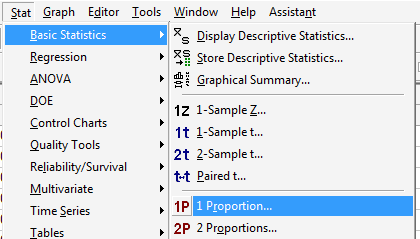
Under the Stat menu, select Basic Statistics, and then 1 Proportion...:
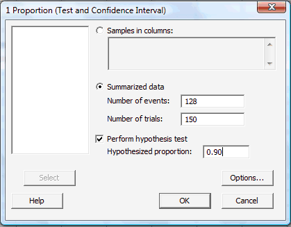
In the pop-up window that appears, click on the radio button labeled Summarized data. In the box labeled Number of events, type in the number of successes or events of interest, and in the box labeled Number of trials, type in the sample size n. Click on the box labeled Perform hypothesis test, and in the box labeled Hypothesized proportion, type in the value of the proportion assumed in the null hypothesis:
Click on the button labeled Options... In the pop-up window that appears, for the box labeled Alternative, select either less than, greater than, or not equal depending on the direction of the alternative hypothesis. Click on the box labeled Use test and interval based on normal distribution:

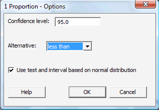
Then, click OK to return to the main pop-up window.

Then, upon clicking OK on the main pop-up window, the output should appear in the Session window:

Test of P = 0.9 vs p < 0.9
Sample	X	N	Sample P	95% Upper Bound	Z-Value	P-Value
1	128	150	0.853333	0.900846	-1.91	0.028

Using the normal approximation.

As you can see, Minitab reports not only the value of the test statistic (Z = −1.91) but also the P-value (0.028) and the 95% confidence interval (one-sided in this case, because of the one-sided hypothesis).

Hypothesis Test for Comparing Two Proportions

To illustrate how to tell Minitab to perform a Z-test for comparing two population proportions, let's refer to the smoker survey example that appeared on the page called Comparing Two Proportions.

Under the Stat menu, select Basic Statistics, and then 2 Proportions...:
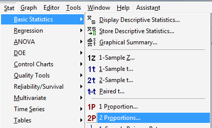
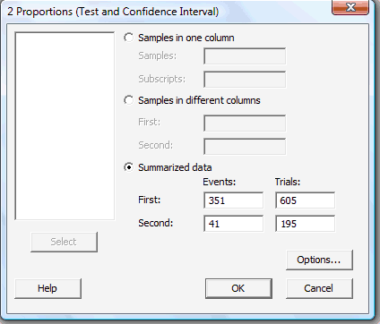
In the pop-up window that appears, click on the radio button labeled Summarized data. In the boxes labeled Events, type in the number of successes or events of interest for both the First and Second samples. And in the boxes labeled Trials, type in the size \(n_1\) of the First sample and the size \(n_2\) of the Second sample:
Click on the button labeled Options... In the pop-up window that appears, in the box labeled Test difference, type in the assumed value of the difference in the proportions that appears in the null hypothesis. The default value is 0.0, the value most commonly assumed, as it means that we are interested in testing for the equality of the population proportions. For the box labeled Alternative, select either less than, greater than, or not equal depending on the direction of the alternative hypothesis. Click on the box labeled Use pooled estimate of p for test:

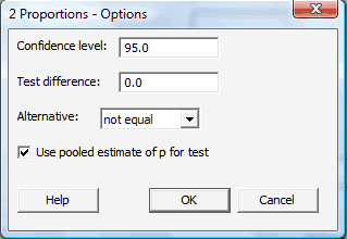
Then, click OK to return to the main pop-up window.
Then, upon clicking OK on the main pop-up window, the output should appear in the Session window:

Sample X N Sample P

1 351 605 0.580165

2 41 195 0.210256

Difference = p (1) - p (2)
Estimate for difference: 0.369909
95% CI for difference: (0.0300499, 0.439319)
T-Test of difference = 0 (vs not =0): Z = 8.99 P-Value = 0.000

Fischer's exact test: P-Value = 0.000

Again, as you can see, Minitab reports not only the value of the test statistic (Z = 8.99) but other useful things as well, including the P-value, which in this case is so small as to be deemed to be 0.000 to three digits. For scientific reporting purposes, we would typically write that as P < 0.0001.

^[1]	Link
↥	Has Tooltip/Popover
	Toggleable Visibility

Sample	X	N	Sample P
1	351	605	0.580165
2	41	195	0.210256

Lesson 9: Tests About Proportions

9.1 - The Basic Idea

Example 9-1

Answer

Example (continued)

Answer

Possible Errors

9.2 - More Examples

Example 9-2

Answer

Example 9-3

Answer

9.3 - The P-Value Approach

Example 9-4

Answer

Example 9-4 (continued)

Answer

Example 9-4 (continued)

Answer

Example 9-4 (continued)

Answer

Note!

Answer

9.4 - Comparing Two Proportions

Example 9-5

Answer

Proof

Example 9-5 (continued)

Answer

Note!

9.5 - Using Minitab

Hypothesis Test for a Single Proportion

Hypothesis Test for Comparing Two Proportions