Lesson 10: Tests About One Mean
Lesson 10: Tests About One MeanOverview
In this lesson, we'll continue our investigation of hypothesis testing. In this case, we'll focus our attention on a hypothesis test for a population mean \(\mu\) for three situations:
- a hypothesis test based on the normal distribution for the mean \(\mu\) for the completely unrealistic situation that the population variance \(\sigma^2\) is known
- a hypothesis test based on the \(t\)-distribution for the mean \(\mu\) for the (much more) realistic situation that the population variance \(\sigma^2\) is unknown
- a hypothesis test based on the \(t\)-distribution for \(\mu_D\), the mean difference in the responses of two dependent populations
10.1 - Z-Test: When Population Variance is Known
10.1 - Z-Test: When Population Variance is KnownLet's start by acknowledging that it is completely unrealistic to think that we'd find ourselves in the situation of knowing the population variance, but not the population mean. Therefore, the hypothesis testing method that we learn on this page has limited practical use. We study it only because we'll use it later to learn about the "power" of a hypothesis test (by learning how to calculate Type II error rates). As usual, let's start with an example.
Example 10-1

Boys of a certain age are known to have a mean weight of \(\mu=85\) pounds. A complaint is made that the boys living in a municipal children's home are underfed. As one bit of evidence, \(n=25\) boys (of the same age) are weighed and found to have a mean weight of \(\bar{x}\) = 80.94 pounds. It is known that the population standard deviation \(\sigma\) is 11.6 pounds (the unrealistic part of this example!). Based on the available data, what should be concluded concerning the complaint?
Answer
The null hypothesis is \(H_0:\mu=85\), and the alternative hypothesis is \(H_A:\mu<85\). In general, we know that if the weights are normally distributed, then:
\(Z=\dfrac{\bar{X}-\mu}{\sigma/\sqrt{n}}\)
follows the standard normal \(N(0,1)\) distribution. It is actually a bit irrelevant here whether or not the weights are normally distributed, because the same size \(n=25\) is large enough for the Central Limit Theorem to apply. In that case, we know that \(Z\), as defined above, follows at least approximately the standard normal distribution. At any rate, it seems reasonable to use the test statistic:
\(Z=\dfrac{\bar{X}-\mu_0}{\sigma/\sqrt{n}}\)
for testing the null hypothesis
\(H_0:\mu=\mu_0\)
against any of the possible alternative hypotheses \(H_A:\mu \neq \mu_0\), \(H_A:\mu<\mu_0\), and \(H_A:\mu>\mu_0\).
For the example in hand, the value of the test statistic is:
\(Z=\dfrac{80.94-85}{11.6/\sqrt{25}}=-1.75\)
The critical region approach tells us to reject the null hypothesis at the \(\alpha=0.05\) level if \(Z<-1.645\). Therefore, we reject the null hypothesis because \(Z=-1.75<-1.645\), and therefore falls in the rejection region:
As always, we draw the same conclusion by using the \(p\)-value approach. Recall that the \(p\)-value approach tells us to reject the null hypothesis at the \(\alpha=0.05\) level if the \(p\)-value \(\le \alpha=0.05\). In this case, the \(p\)-value is \(P(Z<-1.75)=0.0401\):
As expected, we reject the null hypothesis because the \(p\)-value \(=0.0401<\alpha=0.05\).
By the way, we'll learn how to ask Minitab to conduct the \(Z\)-test for a mean \(\mu\) in a bit, but this is what the Minitab output for this example looks like this:
| N | Mean | SE Mean | 95% Upper Bound | Z | P |
|---|---|---|---|---|---|
| 25 | 80.9400 | 2.3200 | 84.7561 | -1.75 | 0.040 |
10.2 - T-Test: When Population Variance is Unknown
10.2 - T-Test: When Population Variance is UnknownNow that, for purely pedagogical reasons, we have the unrealistic situation (of a known population variance) behind us, let's turn our attention to the realistic situation in which both the population mean and population variance are unknown.
Example 10-2

It is assumed that the mean systolic blood pressure is \(\mu\) = 120 mm Hg. In the Honolulu Heart Study, a sample of \(n=100\) people had an average systolic blood pressure of 130.1 mm Hg with a standard deviation of 21.21 mm Hg. Is the group significantly different (with respect to systolic blood pressure!) from the regular population?
Answer
The null hypothesis is \(H_0:\mu=120\), and because there is no specific direction implied, the alternative hypothesis is \(H_A:\mu\ne 120\). In general, we know that if the data are normally distributed, then:
\(T=\dfrac{\bar{X}-\mu}{S/\sqrt{n}}\)
follows a \(t\)-distribution with \(n-1\) degrees of freedom. Therefore, it seems reasonable to use the test statistic:
\(T=\dfrac{\bar{X}-\mu_0}{S/\sqrt{n}}\)
for testing the null hypothesis \(H_0:\mu=\mu_0\) against any of the possible alternative hypotheses \(H_A:\mu \neq \mu_0\), \(H_A:\mu<\mu_0\), and \(H_A:\mu>\mu_0\). For the example in hand, the value of the test statistic is:
\(t=\dfrac{130.1-120}{21.21/\sqrt{100}}=4.762\)
The critical region approach tells us to reject the null hypothesis at the \(\alpha=0.05\) level if \(t\ge t_{0.025, 99}=1.9842\) or if \(t\le t_{0.025, 99}=-1.9842\). Therefore, we reject the null hypothesis because \(t=4.762>1.9842\), and therefore falls in the rejection region:
Again, as always, we draw the same conclusion by using the \(p\)-value approach. The \(p\)-value approach tells us to reject the null hypothesis at the \(\alpha=0.05\) level if the \(p\)-value \(\le \alpha=0.05\). In this case, the \(p\)-value is \(2 \times P(T_{99}>4.762)<2\times P(T_{99}>1.9842)=2(0.025)=0.05\):
As expected, we reject the null hypothesis because \(p\)-value \(\le 0.01<\alpha=0.05\).
Again, we'll learn how to ask Minitab to conduct the t-test for a mean \(\mu\) in a bit, but this is what the Minitab output for this example looks like:
| N | Mean | StDev | SE Mean | 95% CI | T | P |
|---|---|---|---|---|---|---|
| 100 | 130.100 | 21.210 | 2.121 | (125.891, 134.309) | 4.76 | 0.000 |
By the way, the decision to reject the null hypothesis is consistent with the one you would make using a 95% confidence interval. Using the data, a 95% confidence interval for the mean \(\mu\) is:
\(\bar{x}\pm t_{0.025,99}\left(\dfrac{s}{\sqrt{n}}\right)=130.1 \pm 1.9842\left(\dfrac{21.21}{\sqrt{100}}\right)\)
which simplifies to \(130.1\pm 4.21\). That is, we can be 95% confident that the mean systolic blood pressure of the Honolulu population is between 125.89 and 134.31 mm Hg. How can a population living in a climate with consistently sunny 80 degree days have elevated blood pressure?!
Anyway, the critical region approach for the \(\alpha=0.05\) hypothesis test tells us to reject the null hypothesis that \(\mu=120\):
if \(t=\dfrac{\bar{x}-\mu_0}{s/\sqrt{n}}\geq 1.9842\) or if \(t=\dfrac{\bar{x}-\mu_0}{s/\sqrt{n}}\leq -1.9842\)
which is equivalent to rejecting:
if \(\bar{x}-\mu_0 \geq 1.9842\left(\dfrac{s}{\sqrt{n}}\right)\) or if \(\bar{x}-\mu_0 \leq -1.9842\left(\dfrac{s}{\sqrt{n}}\right)\)
which is equivalent to rejecting:
if \(\mu_0 \leq \bar{x}-1.9842\left(\dfrac{s}{\sqrt{n}}\right)\) or if \(\mu_0 \geq \bar{x}+1.9842\left(\dfrac{s}{\sqrt{n}}\right)\)
which, upon inserting the data for this particular example, is equivalent to rejecting:
if \(\mu_0 \leq 125.89\) or if \(\mu_0 \geq 134.31\)
which just happen to be (!) the endpoints of the 95% confidence interval for the mean. Indeed, the results are consistent!
10.3 - Paired T-Test
10.3 - Paired T-TestIn the next lesson, we'll learn how to compare the means of two independent populations, but there may be occasions in which we are interested in comparing the means of two dependent populations. For example, suppose a researcher is interested in determining whether the mean IQ of the population of first-born twins differs from the mean IQ of the population of second-born twins. She identifies a random sample of \(n\) pairs of twins, and measures \(X\), the IQ of the first-born twin, and \(Y\), the IQ of the second-born twin. In that case, she's interested in determining whether:
\(\mu_X=\mu_Y\)
or equivalently if:
\(\mu_X-\mu_Y=0\)
Now, the population of first-born twins is not independent of the population of second-born twins. Since all of our distributional theory requires the independence of measurements, we're rather stuck. There's a way out though... we can "remove" the dependence between \(X\) and \(Y\) by subtracting the two measurements \(X_i\) and \(Y_i\) for each pair of twins \(i\), that is, by considering the independent measurements
\(D_i=X_i-Y_i\)
Then, our null hypothesis involves just a single mean, which we'll denote \(\mu_D\), the mean of the differences:
\(H_0=\mu_D=\mu_X-\mu_Y=0\)
and then our hard work is done! We can just use the \(t\)-test for a mean for conducting the hypothesis test... it's just that, in this situation, our measurements are differences \(d_i\) whose mean is \(\bar{d}\) and standard deviation is \(s_D\). That is, when testing the null hypothesis \(H_0:\mu_D=\mu_0\) against any of the alternative hypotheses \(H_A:\mu_D \neq \mu_0\), \(H_A:\mu_D<\mu_0\), and \(H_A:\mu_D>\mu_0\), we compare the test statistic:
\(t=\dfrac{\bar{d}-\mu_0}{s_D/\sqrt{n}}\)
to a \(t\)-distribution with \(n-1\) degrees of freedom. Let's take a look at an example!
Example 10-3

Blood samples from \(n=10\) = 10 people were sent to each of two laboratories (Lab 1 and Lab 2) for cholesterol determinations. The resulting data are summarized here:
| Subject | Lab 1 | Lab 2 | Diff |
|---|---|---|---|
|
1 |
296 | 318 | -22 |
| 2 | 268 | 287 | -19 |
| . | . | . | . |
| . | . | . | . |
| . | . | . | . |
| 10 | 262 | 285 | -23 |
| \(\bar{x}_{1}=260.6\) | \(\bar{x}_{2}=275\) | \(\begin{array}{c} \bar{d}=-14.4 \\ s_{d}=6.77 \end{array}\) |
Is there a statistically significant difference at the \(\alpha=0.01\) level, say, in the (population) mean cholesterol levels reported by Lab 1 and Lab 2?
Answer
The null hypothesis is \(H_0:\mu_D=0\), and the alternative hypothesis is \(H_A:\mu_D\ne 0\). The value of the test statistic is:
\(t=\dfrac{-14.4-0}{6.77/\sqrt{10}}=-6.73\)
The critical region approach tells us to reject the null hypothesis at the \(\alpha=0.01\) level if \(t>t_{0.005, 9}=3.25\) or if \(t<t_{0.005, 9}=-3.25\). Therefore, we reject the null hypothesis because \(t=-6.73<-3.25\), and therefore falls in the rejection region.
Again, we draw the same conclusion when using the \(p\)-value approach. In this case, the \(p\)-value is:
\(p-\text{value }=2\times P(T_9<-6.73)\le 2\times 0.005=0.01\)
As expected, we reject the null hypothesis because \(p\)-value \(\le 0.01=\alpha\).
And, the Minitab output for this example looks like this:
| N | Mean | StDev | SE Mean | 95% CI | T | P |
|---|---|---|---|---|---|---|
| 10 | -14.4000 | 6.7700 | 2.1409 | (-19.2430, -9.5570) | -6.73 | 0.000 |
10.4 - Using Minitab
10.4 - Using MinitabZ-Test for a Single Mean
To illustrate how to tell Minitab to perform a Z-test for a single mean, let's refer to the boys weight example that appeared on the page called The Z-test: When Population Variance is Known.
-
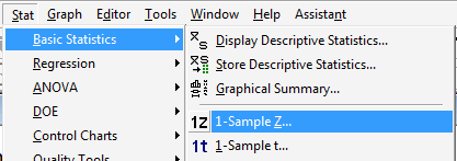
Under the Stat menu, select Basic Statistics, and then 1-Sample Z...:
-
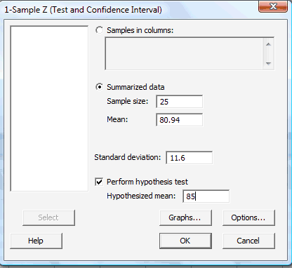
In the pop-up window that appears, click on the radio button labeled Summarized data. In the box labeled Sample size, type in the sample size n, and in the box labeled Mean, type in the sample mean. In the box labeled Standard deviation, type in the value of the known (or rather assumed!) population standard deviation. Click on the box labeled Perform hypothesis test, and in the box labeled Hypothesized mean, type in the value of the mean assumed in the null hypothesis:
-
Click on the button labeled Options... In the pop-up window that appears, for the box labeled Alternative, select either less than, greater than, or not equal depending on the direction of the alternative hypothesis:

Then, click OK to return to the main pop-up window.
-
Then, upon clicking OK on the main pop-up window, the output should appear in the Session window:
Test of mu = 85 vs < 85
The assumed standard deviation = 11.6N Mean SE Mean 95% Upper Bound Z P 25 80.94 2.32 84.76 -1.75 0.040
T-test for a Single Mean
To illustrate how to tell Minitab to perform a t-test for a single mean, let's refer to the systolic blood pressure example that appeared on the page called The T-test: When Population Variance is Unknown.
-
Under the Stat menu, select Basic Statistics, and then 1-Sample t...:

-
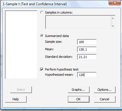
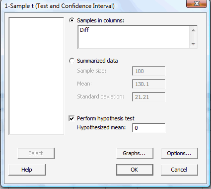
In the pop-up window that appears, click on the radio button labeled Summarized data. In the box labeled Sample size, type in the sample size n; in the box labeled Mean, type in the sample mean; and in the box labeled Standard deviation, type in the sample standard deviation. Click on the box labeled Perform hypothesis test, and in the box labeled Hypothesized mean, type in the value of the mean assumed in the null hypothesis:
-
Click on the button labeled Options... In the pop-up window that appears, for the box labeled Alternative, select either less than, greater than, or not equal depending on the direction of the alternative hypothesis:

Then, click OK to return to the main pop-up window.
-
Then, upon clicking OK on the main pop-up window, the output should appear in the Session window:
Test of mu = 120 vs not = 120 N Mean StDev SE Mean 95% CI T P 100 130.10 21.21 2.12 (125.89, 134.31) 4.76 0.000 (5) Note that a paired t-test can be performed in the same way. The summarized sample data would simply be the summarized differences. The extra step of calculating the differences would be required, however, if your data are the raw measurements from the two dependent samples. That is, if you have two columns containing, say, Before and After measurements for which you want to analyze Diff, their differences, you can use Minitab's calculator (under the Calc menu, select Calculator) to calculate the differences:
-
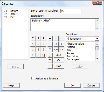
Upon clicking OK, the differences (Diff) should appear in your worksheet:
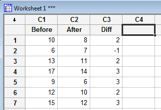
When performing the t-test, you'll then need to tell Minitab (in the Samples in columns box) that the differences are contained in the Diff column:
Here's what the paired t-test output would look like for this example:
One Sample T: Diff
Test of mu = 0 vs not = 0Variable N Mean StDev SE Mean 95% CI T P Diff 7 2.000 1.414 0.535 (0.692, 3.308) 3.74 0.010