Lesson 11: Tests of the Equality of Two Means
Lesson 11: Tests of the Equality of Two MeansOverview
In this lesson, we'll continue our investigation of hypothesis testing. In this case, we'll focus our attention on a hypothesis test for the difference in two population means \(\mu_1-\mu_2\) for two situations:
- a hypothesis test based on the \(t\)-distribution, known as the pooled two-sample \(t\)-test, for \(\mu_1-\mu_2\) when the (unknown) population variances \(\sigma^2_X\) and \(\sigma^2_Y\) are equal
- a hypothesis test based on the \(t\)-distribution, known as Welch's \(t\)-test, for \(\mu_1-\mu_2\) when the (unknown) population variances \(\sigma^2_X\) and \(\sigma^2_Y\) are not equal
Of course, because population variances are generally not known, there is no way of being 100% sure that the population variances are equal or not equal. In order to be able to determine, therefore, which of the two hypothesis tests we should use, we'll need to make some assumptions about the equality of the variances based on our previous knowledge of the populations we're studying.
11.1 - When Population Variances Are Equal
11.1 - When Population Variances Are EqualLet's start with the good news, namely that we've already done the dirty theoretical work in developing a hypothesis test for the difference in two population means \(\mu_1-\mu_2\) when we developed a \((1-\alpha)100\%\) confidence interval for the difference in two population means. Recall that if you have two independent samples from two normal distributions with equal variances \(\sigma^2_X=\sigma^2_Y=\sigma^2\), then:
\(T=\dfrac{(\bar{X}-\bar{Y})-(\mu_X-\mu_Y)}{S_p\sqrt{\dfrac{1}{n}+\dfrac{1}{m}}}\)
follows a \(t_{n+m-2}\) distribution where \(S^2_p\), the pooled sample variance:
\(S_p^2=\dfrac{(n-1)S^2_X+(m-1)S^2_Y}{n+m-2}\)
is an unbiased estimator of the common variance \(\sigma^2\). Therefore, if we're interested in testing the null hypothesis:
\(H_0:\mu_X-\mu_Y=0\) (or equivalently \(H_0:\mu_X=\mu_Y\))
against any of the alternative hypotheses:
\(H_A:\mu_X-\mu_Y \neq 0,\quad H_A:\mu_X-\mu_Y < 0,\text{ or }H_A:\mu_X-\mu_Y > 0\)
we can use the test statistic:
\(T=\dfrac{(\bar{X}-\bar{Y})-(\mu_X-\mu_Y)}{S_p\sqrt{\dfrac{1}{n}+\dfrac{1}{m}}}\)
and follow the standard hypothesis testing procedures. Let's take a look at an example.
Example 11-1

A psychologist was interested in exploring whether or not male and female college students have different driving behaviors. There were several ways that she could quantify driving behaviors. She opted to focus on the fastest speed ever driven by an individual. Therefore, the particular statistical question she framed was as follows:
Is the mean fastest speed driven by male college students different than the mean fastest speed driven by female college students?
She conducted a survey of a random \(n=34\) male college students and a random \(m=29\) female college students. Here is a descriptive summary of the results of her survey:
| Males (X) | Females (Y) |
|---|---|
|
\(n = 34\) |
\(m = 29\) \(\bar{y} = 90.9\) \(s_y = 12.2\) |
and here is a graphical summary of the data in the form of a dotplot:
Is there sufficient evidence at the \(\alpha=0.05\) level to conclude that the mean fastest speed driven by male college students differs from the mean fastest speed driven by female college students?
Answer
Because the observed standard deviations of the two samples are of similar magnitude, we'll assume that the population variances are equal. Let's also assume that the two populations of fastest speed driven for males and females are normally distributed. (We can confirm, or deny, such an assumption using a normal probability plot, but let's simplify our analysis for now.) The randomness of the two samples allows us to assume independence of the measurements as well.
Okay, assumptions all met, we can test the null hypothesis:
\(H_0:\mu_M-\mu_F=0\)
against the alternative hypothesis:
\(H_A:\mu_M-\mu_F \neq 0\)
using the test statistic:
\(t=\dfrac{(105.5-90.9)-0}{16.9 \sqrt{\dfrac{1}{34}+\dfrac{1}{29}}}=3.42\)
because, among other things, the pooled sample standard deviation is:
\(s_p=\sqrt{\dfrac{33(20.1^2)+28(12.2^2)}{61}}=16.9\)
The critical value approach tells us to reject the null hypothesis in favor of the alternative hypothesis if:
\(|t|\geq t_{\alpha/2,n+m-2}=t_{0.025,61}=1.9996\)
We reject the null hypothesis because the test statistic (\(t=3.42\)) falls in the rejection region:
There is sufficient evidence at the \(\alpha=0.05\) level to conclude that the average fastest speed driven by the population of male college students differs from the average fastest speed driven by the population of female college students.
Not surprisingly, the decision is the same using the \(p\)-value approach. The \(p\)-value is 0.0012:
\(P=2\times P(T_{61}>3.42)=2(0.0006)=0.0012\)
Therefore, because \(p=0.0012\le \alpha=0.05\), we reject the null hypothesis in favor of the alternative hypothesis. Again, we conclude that there is sufficient evidence at the \(\alpha=0.05\) level to conclude that the average fastest speed driven by the population of male college students differs from the average fastest speed driven by the population of female college students.
By the way, we'll see how to tell Minitab to conduct a two-sample t-test in a bit here, but in the meantime, this is what the output would look like:
Two-Sample T: For Fastest
| Gender | N | Mean | StDev | SE Mean |
|---|---|---|---|---|
| 1 | 34 | 105.5 | 20.1 | 3.4 |
| 2 | 29 | 90.9 | 12.2 | 2.3 |
Difference = mu (1) - mu (2)
Estimate for difference: 14.6085
95% CI for difference: (6.0630, 23.1540)
T-Test of difference = 0 (vs not =) : T-Value = 3.42 P-Value = 0.001 DF = 61
Both use Pooled StDev = 16.9066
11.2 - When Population Variances Are Not Equal
11.2 - When Population Variances Are Not EqualLet's again start with the good news that we've already done the dirty theoretical work here. Recall that if you have two independent samples from two normal distributions with unequal variances \(\sigma^2_X \neq \sigma^2_Y\), then:
\(T=\dfrac{(\bar{X}-\bar{Y})-(\mu_X-\mu_Y)}{\sqrt{\dfrac{S^2_X}{n}+\dfrac{S^2_Y}{m}}}\)
follows, at least approximately, a \(t_r\) distribution where \(r\), the adjusted degrees of freedom is determined by the equation:
\(r=\dfrac{\left(\dfrac{s^2_X}{n}+\dfrac{s^2_Y}{m}\right)^2}{\dfrac{(s^2_X/n)^2}{n-1}+\dfrac{(s^2_Y/m)^2}{m-1}}\)
If r doesn't equal an integer, as it usually doesn't, then we take the integer portion of \(r\). That is, we use \(\lfloor r\rfloor\) if necessary.
With that now being recalled, if we're interested in testing the null hypothesis:
\(H_0:\mu_X-\mu_Y=0\) (or equivalently \(H_0:\mu_X=\mu_Y\))
against any of the alternative hypotheses:
\(H_A:\mu_X-\mu_Y \neq 0,\quad H_A:\mu_X-\mu_Y < 0,\text{ or }H_A:\mu_X-\mu_Y > 0\)
we can use the test statistic:
\(T=\dfrac{(\bar{X}-\bar{Y})-(\mu_X-\mu_Y)}{\sqrt{\dfrac{S^2_X}{n}+\dfrac{S^2_Y}{m}}}\)
and follow the standard hypothesis testing procedures. Let's return to our fastest speed driven example.
Example 11-1 (Continued)

A psychologist was interested in exploring whether or not male and female college students have different driving behaviors. There were a number of ways that she could quantify driving behaviors. She opted to focus on the fastest speed ever driven by an individual. Therefore, the particular statistical question she framed was as follows:
Is the mean fastest speed driven by male college students different than the mean fastest speed driven by female college students?
She conducted a survey of a random \(n=34\) male college students and a random \(m=29\) female college students. Here is a descriptive summary of the results of her survey:
| Males (X) | Females (Y) |
|---|---|
|
\(n = 34\) |
\(m = 29\) \(\bar{y} = 90.9\) \(s_y = 12.2\) |
Is there sufficient evidence at the \(\alpha=0.05\) level to conclude that the mean fastest speed driven by male college students differs from the mean fastest speed driven by female college students?
Answer
This time let's not assume that the population variances are equal. Then, we'll see if we arrive at a different conclusion. Let's still assume though that the two populations of fastest speed driven for males and females are normally distributed. And, we'll again permit the randomness of the two samples to allow us to assume independence of the measurements as well.
That said, then we can test the null hypothesis:
\(H_0:\mu_M-\mu_F=0\)
against the alternative hypothesis:
\(H_A:\mu_M-\mu_F \neq 0\)
comparing the test statistic:
\(t=\dfrac{(105.5-90.9)-0}{\sqrt{\dfrac{20.1^2}{34}+\dfrac{12.2^2}{29}}}=3.54\)
to a \(T\) distribution with \(r\) degrees of freedom, where:
\(r=\dfrac{\left(\dfrac{12.2^2}{29}+\dfrac{20.1^2}{34} \right)^2}{\left( \dfrac{1}{28}\right)\left(\dfrac{12.2^2}{29} \right)^2+\left(\dfrac{1}{33}\right)\left(\dfrac{20.1^2}{34} \right)^2}=55.5\)
Oops... that's not an integer, so we're going to need to take the greatest integer portion of that \(r\). That is, we take the degrees of freedom to be \(\lfloor r\rfloor = \lfloor 55.5\rfloor=55\).
Then, the critical value approach tells us to reject the null hypothesis in favor of the alternative hypothesis if:
\(t>t_{0.025,55}=2.004\)
We reject the null hypothesis because the test statistic (\(t=3.54\)) falls in the rejection region:
There is (again!) sufficient evidence at the \(\alpha=0.05\) level to conclude that the average fastest speed driven by the population of male college students differs from the average fastest speed driven by the population of female college students.
And again, the decision is the same using the \(p\)-value approach. The \(p\)-value is 0.0008:
\(P=2\times P(T_{55}>3.54)=2(0.0004)=0.0008\)
Therefore, because \(p=0.008\le \alpha=0.05\), we reject the null hypothesis in favor of the alternative hypothesis. Again, we conclude that there is sufficient evidence at the \(\alpha=0.05\) level to conclude that the average fastest speed driven by the population of male college students differs from the average fastest speed driven by the population of female college students.
At any rate, we see that in this case, our conclusion is the same regardless of whether or not we assume equality of the population variances.
And, just in case you're interested... we'll see how to tell Minitab to conduct a Welch's \(t\)-test very soon, but in the meantime, this is what the output would look like for this example:
Two-Sample T: For Fastest
| Gender | N | Mean | StDev | SE Mean |
|---|---|---|---|---|
| 1 | 34 | 105.5 | 20.1 | 3.4 |
| 2 | 29 | 90.9 | 12.2 | 2.3 |
Difference = mu (1) - mu (2)
Estimate for difference: 14.6085
95% CI for difference: (6.3575, 22.8596)
T-Test of difference = 0 (vs not =) : T-Value = 3.55 P-Value = 0.001 DF = 55
11.3 - Using Minitab
11.3 - Using MinitabJust as is the case for asking Minitab to calculate pooled t-intervals and Welch's t-intervals for \(\mu_1-\mu_2\), the commands necessary for asking Minitab to perform a two-sample t-test or a Welch's t-test depend on whether the data are entered in two columns, or the data are entered in one column with a grouping variable in a second column.
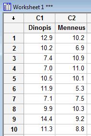
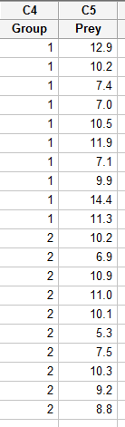
Let's recall the spider and prey example, in which the feeding habits of two species of net-casting spiders were studied. The species, the deinopis, and menneus coexist in eastern Australia. The following data were obtained on the size, in millimeters, of the prey of random samples of the two species:
| sample 1 | sample 2 | sample 3 | sample 4 | sample 5 | sample 6 | sample 7 | sample 8 | sample 9 | sample 10 |
|---|---|---|---|---|---|---|---|---|---|
| 12.9 | 10.2 | 7.4 | 7.0 | 10.5 | 11.9 | 7.1 | 9.9 | 14.4 | 11.3 |
| sample 1 | sample 2 | sample 3 | sample 4 | sample 5 | sample 6 | sample 7 | sample 8 | sample 9 | sample 10 |
|---|---|---|---|---|---|---|---|---|---|
| 10.2 | 6.9 | 10.9 | 11.0 | 10.1 | 5.3 | 7.5 | 10.3 | 9.2 | 8.8 |
Let's use the data and Minitab to test whether the mean prey size of the populations of the two types of spiders differs.
When the Data are Entered in Two Columns
-
Enter the data in two columns, such as:
-
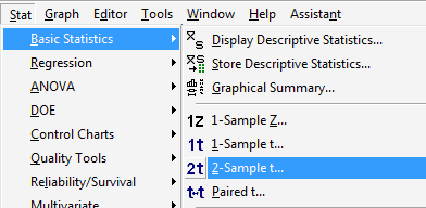
Under the Stat menu, select Basic Statistics, and then select 2-Sample t...:
-
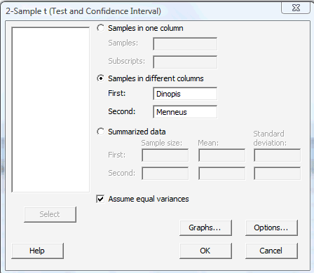
In the pop-up window that appears, select Samples in different columns. Specify the name of the First variable, and specify the name of the Second variable. For the two-sample (pooled) t-test, click on the box labeled Assume equal variances. (For Welch's t-test, leave the box labeled Assume equal variances unchecked.):
-
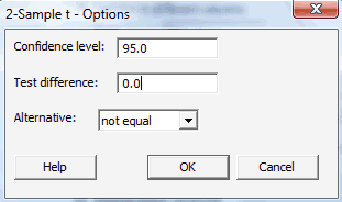
Click on the button labeled Options... In the pop-up window that appears, for the box labeled Alternative, select either less than, greater than, or not equal depending on the direction of the alternative hypothesis:
Then, click OK to return to the main pop-up window.
-
Then, upon clicking OK on the main pop-up window, the output should appear in the Session window:
Two-Sample T: For Deinopis vs Menneus Variable N Mean StDev SE Mean Deinopis 10 10.26 2.51 0.79 Menneus 10 9.02 1.90 0.60 Difference = mu (Deinopis) - mu (Menneus)
Estimate for difference: 1.240
95% CI for difference: (-0.852, 3.332)
T-Test of difference = 0 (vs not =): T-Value = 1.25 P-Value = 0.229 DF = 18
Both use Pooled StDev = 2.2266
When the Data are Entered in One Column, and a Grouping Variable in a Second Column
-
Enter the data in one column (called Prey, say), and the grouping variable in a second column (called Group, say, with 1 denoting a deinopis spider and 2 denoting a menneus spider), such as:
-
Under the Stat menu, select Basic Statistics, and then select 2-Sample t...:
-
In the pop-up window that appears, select Samples in one column. Specify the name of the Samples variable (Prey, for us) and specify the name of the Subscripts (grouping) variable (Group, for us). For the two-sample (pooled) t-test, click on the box labeled Assume equal variances. (For Welch's t-test, leave the box labeled Assume equal variances unchecked.):
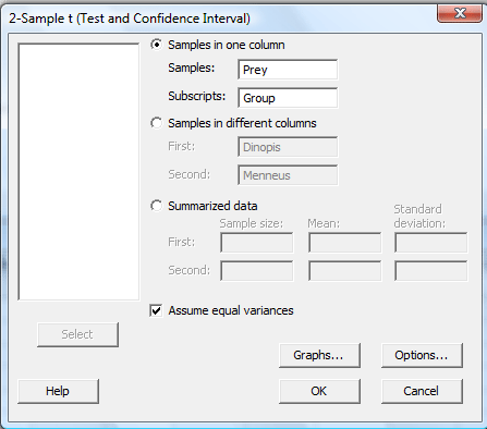
-
Click on the button labeled Options... In the pop-up window that appears, for the box labeled Alternative, select either less than, greater than, or not equal depending on the direction of the alternative hypothesis:
Then, click OK to return to the main pop-up window.
-
Then, upon clicking OK on the main pop-up window, the output should appear in the Session window:
Two-Sample T: For Prey
Group N Mean StDev SE Mean 1 10 10.26 2.51 0.79 2 10 9.02 1.90 0.60 Difference = mu (1) - mu (2)
Estimate for difference: 1.240
95% CI for difference: (-0.852, 3.332)
T-Test of difference = 0 (vs not =): T-Value = 1.25 P-Value = 0.229 DF = 18
Both use Pooled StDev = 2.2266