Yeehah again! The theoretical work for developing a hypothesis test for a population variance \(\sigma^2\) is already behind us. Recall that if you have a random sample of size n from a normal population with (unknown) mean \(\mu\) and variance \(\sigma^2\), then:

\(\chi^2=\dfrac{(n-1)S^2}{\sigma^2}\)

follows a chi-square distribution with n−1 degrees of freedom. Therefore, if we're interested in testing the null hypothesis:

\(H_0 \colon \sigma^2=\sigma^2_0\)

against any of the alternative hypotheses:

\(H_A \colon\sigma^2 \neq \sigma^2_0,\quad H_A \colon\sigma^2<\sigma^2_0,\text{ or }H_A \colon\sigma^2>\sigma^2_0\)

we can use the test statistic:

\(\chi^2=\dfrac{(n-1)S^2}{\sigma^2_0}\)

and follow the standard hypothesis testing procedures. Let's take a look at an example.

Let's now recall the theory necessary for developing a hypothesis test for testing the equality of two population variances. Suppose \(X_1 , X_2 , \dots, X_n\) is a random sample of size n from a normal population with mean \(\mu_X\) and variance \(\sigma^2_X\). And, suppose, independent of the first sample, \(Y_1 , Y_2 , \dots, Y_m\) is another random sample of size m from a normal population with \(\mu_Y\) and variance \(\sigma^2_Y\). Recall then, in this situation, that:

\(\dfrac{(n-1)S^2_X}{\sigma^2_X} \text{ and } \dfrac{(m-1)S^2_Y}{\sigma^2_Y}\)

have independent chi-square distributions with n−1 and m−1 degrees of freedom, respectively. Therefore:

\( {\displaystyle F=\frac{\left[\frac{\color{red}\cancel {\color{black}(n-1)} \color{black}S_{X}^{2}}{\sigma_{x}^{2}} /\color{red}\cancel {\color{black}(n- 1)}\color{black}\right]}{\left[\frac{\color{red}\cancel {\color{black}(m-1)} \color{black}S_{Y}^{2}}{\sigma_{Y}^{2}} /\color{red}\cancel {\color{black}(m-1)}\color{black}\right]}=\frac{S_{X}^{2}}{S_{Y}^{2}} \cdot \frac{\sigma_{Y}^{2}}{\sigma_{X}^{2}}} \)

follows an F distribution with n−1 numerator degrees of freedom and m−1 denominator degrees of freedom. Therefore, if we're interested in testing the null hypothesis:

\(H_0 \colon \sigma^2_X=\sigma^2_Y\) (or equivalently \(H_0 \colon\dfrac{\sigma^2_Y}{\sigma^2_X}=1\))

against any of the alternative hypotheses:

\(H_A \colon \sigma^2_X \neq \sigma^2_Y,\quad H_A \colon \sigma^2_X >\sigma^2_Y,\text{ or }H_A \colon \sigma^2_X <\sigma^2_Y\)

we can use the test statistic:

\(F=\dfrac{S^2_X}{S^2_Y}\)

and follow the standard hypothesis testing procedures. When doing so, we might also want to recall this important fact about the F-distribution:

\(F_{1-(\alpha/2)}(n-1,m-1)=\dfrac{1}{F_{\alpha/2}(m-1,n-1)}\)

so that when we use the critical value approach for a two-sided alternative:

\(H_A \colon\sigma^2_X \neq \sigma^2_Y\)

we reject if the test statistic F is too large:

\(F \geq F_{\alpha/2}(n-1,m-1)\)

or if the test statistic F is too small:

\(F \leq F_{1-(\alpha/2)}(n-1,m-1)=\dfrac{1}{F_{\alpha/2}(m-1,n-1)}\)

Okay, let's take a look at an example. In the last lesson, we performed a two-sample t-test (as well as Welch's test) to test whether the mean fastest speed driven by the population of male college students differs from the mean fastest speed driven by the population of female college students. When we performed the two-sample t-test, we just assumed the population variances were equal. Let's revisit that example again to see if our assumption of equal variances is valid.

In each case, we'll illustrate how to perform the hypothesis tests of this lesson using summarized data.

1. Under the Stat menu, select Basic Statistics, and then select 1 Variance...:

   

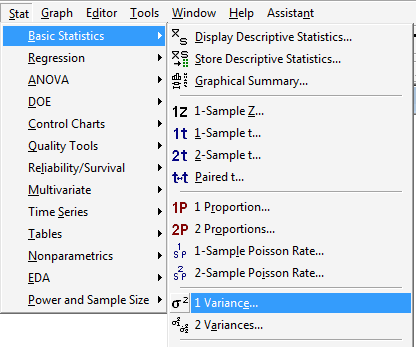
2. In the pop-up window that appears, in the box labeled Data, select Sample standard deviation (or alternatively Sample variance). In the box labeled Sample size, type in the size n of the sample. In the box labeled Sample standard deviation, type in the sample standard deviation. Click on the box labeled Perform hypothesis test, and in the box labeled Value, type in the Hypothesized standard deviation (or alternatively the Hypothesized variance):

   

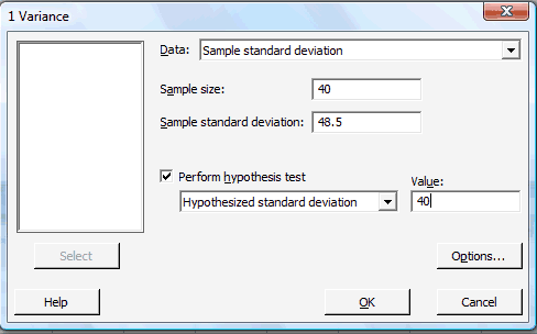
3. Click on the button labeled Options... In the pop-up window that appears, for the box labeled Alternative, select either less than, greater than, or not equal depending on the direction of the alternative hypothesis:

   

   Then, click on OK to return to the main pop-up window.

4. Then, upon clicking OK on the main pop-up window, the output should appear in the Session window:

   95% Confidence Intervals

   Method	CI for StDev	CI for Variance
   Chi-Square	(39.7,  62.3)	(1578,  3878)

   Tests

   Method	Test Statistic	DF	P-Value
   Chi-Square	57.34	39	0.059

    

1. Under the Stat menu, select Basic Statistics, and then select 2 Variances...:

   

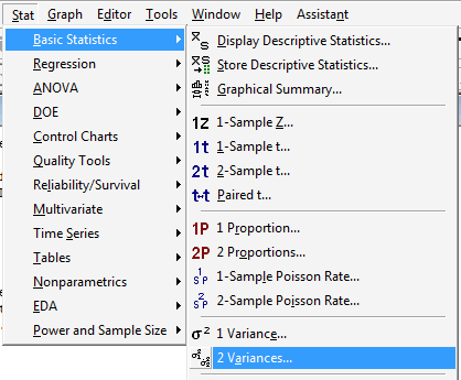
2. In the pop-up window that appears, in the box labeled Data, select Sample standard deviations (or alternatively Sample variances). In the box labeled Sample size, type in the size n of the First sample and m of the Second sample. In the box labeled Standard deviation, type in the sample standard deviations for the First and Second samples:

   

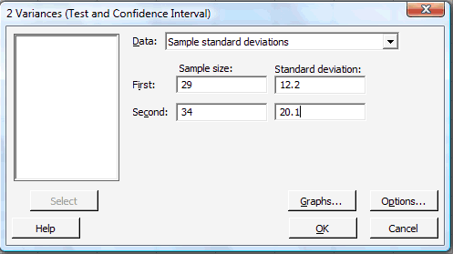
3. Click on the button labeled Options... In the pop-up window that appears, in the box labeled Value, type in the Hypothesized ratio of the standard deviations (or the Hypothesized ratio of the variances). For the box labeled Alternative, select either less than, greater than, or not equal depending on the direction of the alternative hypothesis:

   

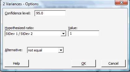
   Then, click on OK to return to the main pop-up window.

   1. Then, upon clicking OK on the main pop-up window, the output should appear in the Session window:

      Test and CI for Two Variances

      Method

      Null hypothesis                 Sigma(1)  /  Sigma(2)  = 1
      Alternative hypothesis     Sigma(1)  /  Sigma(2)  not  = 1
      Significance level              Alpha  =  0.05

      
      Statistics

      Sample	N	StDev	Variance
      1	29	12.200	148.840
      2	34	20.100	404.010

      Ratio of standard deviations  =  0.607
      Ratio of variances  =  0.368

      
      95% Confidence Intervals 

      Distribution of Data	CI for StDev Ratio	CI for Variance Ratio
      Normal	(0.425,  0.877)	(0.180,  0.770)

      Tests

      Method	DF1	DF2	Test Statistic	P-Value
      F Test (normal)	28	33	0.37	0.009