Lesson 18: Order Statistics
Lesson 18: Order StatisticsOverview
We typically don't pay particular attention to the order of a set of random variables \(X_1, X_2, \cdots, X_n\). But, what if we did? Suppose, for example, we needed to know the probability that the third largest value was less than 72. Or, suppose we needed to know the 80th percentile of a random sample of heart rates. In either case, we'd need to know something about how the order of the data behaved. That is, we'd need to know something about the probability density function of the order statistics \(Y_1, Y_2, \cdots, Y_n\). That's what we'll groove on in this lesson.
Objectives
- To learn the formal definition of order statistics.
- To derive the distribution function of the \(r^{th}\) order statistic.
- To derive the probability density function of the \(r^{th}\) order statistic.
- To derive a method for finding the \((100p)^{th}\) percentile of the sample.
18.1 - The Basics
18.1 - The BasicsExample 18-1

Let's motivate the definition of a set of order statistics by way of a simple example.
Suppose a random sample of five rats yields the following weights (in grams):
\(x_1=602 \qquad x_2=781\qquad x_3=709\qquad x_4=742\qquad x_5=633\)
What are the observed order statistics of this set of data?
Answer
Well, without even knowing the formal definition of an order statistic, we probably don't need a rocket scientist to tell us that, in order to find the order statistics, we should probably arrange the data in increasing numerical order. Doing so, the observed order statistics are:
\(y_1=602<y_2=633<y_3=709<y_4=742<y_5=781\)
The only thing that might have tripped us up a bit in such a trivial example is if two of the rats had shared the same weight, as observing ties is certainly a possibility. We'll wash our hands of the likelihood of that happening, though, by making an assumption that will hold throughout this lesson... and beyond. We will assume that the n independent observations come from a continuous distribution, thereby making the probability zero that any two observations are equal. Of course, ties are still possible in practice. Making the assumption, though, that there is a near zero chance of a tie happening allows us to develop the distribution theory of order statistics that hold at least approximately even in the presence of ties. That said, let's now formally provide a definition for a set of order statistics.
Definition. If \(X_1, X_2, \cdots, X_n\) are observations of a random sample of size \(n\) from a continuous distribution, we let the random variables:
\(Y_1<Y_2<\cdots<Y_n\)
denote the order statistics of the sample, with:
- \(Y_1\) being the smallest of the \(X_1, X_2, \cdots, X_n\) observations
- \(Y_2\) being the second smallest of the \(X_1, X_2, \cdots, X_n\) observations
- ....
- \(Y_{n-1}\) being the next-to-largest of the \(X_1, X_2, \cdots, X_n\) observations
- \(Y_n\) being the largest of the \(X_1, X_2, \cdots, X_n\) observations
Now, what we want to do is work our way up to find the probability density function of any of the \(n\) order statistics, the \(r^{th}\) order statistic \(Y_r\). That way, we'd know how the order statistics behave and therefore could use that knowledge to draw conclusions about something like the fastest automobile in a race or the heaviest mouse on a certain diet. In finding the probability density function, we'll use the distribution function technique to do so. It's probably been a mighty bit since we used the technique, so in case you need a reminder, our strategy will be to first find the distribution function \(G_r(y)\) of the \(r^{th}\) order statistic, and then take its derivative to find the probability density function \(g_r(y)\) of the \(r^{th}\) order statistic. We're getting a little bit ahead of ourselves though. That's what we'll do on the next page. To make our work there more understandable, let's first take a look at a concrete example here.
Example 18-2
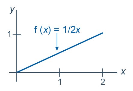
Let \(Y_1<Y_2<Y_3<Y_4<Y_5<Y_6\) be the order statistics associated with \(n=6\) independent observations each from the distribution with probability density function:
\(f(x)=\dfrac{1}{2}x\)
for \(0<x<2\). What is the probability that the next-to-largest order statistic, that is, \(Y_5\), is less than 1? That is, what is \(P(Y_5<1)\)?
Answer
The key to finding the desired probability is to recognize that the only way that the fifth order statistic, \(Y_5\), would be less than one is if at least 5 of the random variables \(X_1, X_2, X_3, X_4, X_5, \text{ and }X_6\) are less than one. For the sake of simplicity, let's suppose the first five observed values \(x_1, x_2, x_3, x_4, x_5\) are less than one, but the sixth \(x_6\) is not. In that case, the observed fifth-order statistic, \(y_5\), would be less than one:

The observed fifth order statistic, \(y_5\), would also be less than one if all six of the observed values \(x_1, x_2, x_3, x_4, x_5, x_6\) are less than one:

The observed fifth order statistic, \(y_5\), would not be less than one if the first four observed values \(x_1, x_2, x_3, x_4\) are less than one, but the fifth \(x_5\) and sixth \(x_6\) is not:

Again, the only way that the fifth order statistic, \(Y_5\), would be less than one is if 5 or 6... that is, at least 5... of the random variables \(X_1, X_2, X_3, X_4, X_5, \text{ and }X_6\) are less than one. For the sake of simplicity, we considered just the first five or six random variables, but in reality, any five or six random variables less than one would do. We just have to do some "choosing" to count the number of ways that we can get any five or six of the random variables to be less than one.
If you think about it, then, we have a binomial probability calculation here. If the event \(\{X_i<1\}\), \(i=1, 2, \cdots, 5\) is considered a "success," and we let \(Z\) = the number of successes in six mutually independent trials, then \(Z\) is a binomial random variable with \(n=6\) and \(p=0.25\):
\(P(X_i\le1)=\dfrac{1}{2}\int_{0}^{1}x dx=\dfrac{1}{2}\left[\dfrac{x^2}{2}\right]_{x=0}^{x=1}=\dfrac{1}{2}\left(\dfrac{1}{2}-0\right)=\dfrac{1}{4}\)
Finding the probability that the fifth order statistic, \(Y_5\), is less than one reduces to a binomial calculation then. That is:
\(P(Y_5<1)=P(Z=5)+P(Z=6)=\binom{6}{5}\left(\dfrac{1}{4} \right)^5\left(\dfrac{3}{4} \right)^1+\binom{6}{6}\left(\dfrac{1}{4} \right)^6\left(\dfrac{3}{4} \right)^0=0.0046\)
The fact that the calculated probability is so small should make sense in light of the given p.d.f. of \(X\). After all, each individual \(X_i\) has a greater chance of falling above, rather than below, one. For that reason, it would unusual to observe as many as five or six \(X\)'s less than one.
What is the cumulative distribution function \(G_5(y)\) of the fifth order statistic \(Y_5\)?
Answer
Recalling the definition of a cumulative distribution function, \(G_5(y)\) is defined to be the probability that the fifth order statistic \(Y_5\) is less than some value \(y\). That is:
\(G_5(y)=P(Y_5 < y)\)
Well, in our above work, we found the probability that the fifth order statistic \(Y_5\) is less than a specific value, namely 1. We just need to generalize our work there to allow for any value \(y\). Well, if the event \(\{X_i<y\}\), \(i=1, 2, \cdots, 5\) is considered a "success," and we let \(Z\) = the number of successes in six mutually independent trials, then \(Z\) is a binomial random variable with \(n=6\) and probability of success:
\(P(X_i\le y)=\dfrac{1}{2}\int_{0}^{y}x dx=\dfrac{1}{2}\left[\dfrac{x^2}{2}\right]_{x=0}^{x=y}=\dfrac{1}{2}\left(\dfrac{y^2}{2}-0\right)=\dfrac{y^2}{4}\)
Therefore, the cumulative distribution function \(G_5(y)\) of the fifth order statistic \(Y_5\) is:
\(G_5(y)=P(Y_5 < y)=P(Z=5)+P(Z=6)=\binom{6}{5}\left(\dfrac{y^2}{4}\right)^5\left(1-\dfrac{y^2}{4}\right)+\left(\dfrac{y^2}{4}\right)^6\)
for \(0<y<2\).
What is the probability density function \(g_5(y)\) of the fifth order statistic \(Y_5\)?
Answer
All we need to do to find the probability density function \(g_{5}(y)\) is to take the derivative of the distribution function \(G_5(y)\) with respect to \(y\). Doing so, we get:
\(g_5(y)=G_{5}^{'}(y)=\binom{6}{5}\left(\dfrac{y^2}{4}\right)^5\left(\dfrac{-2y}{4}\right)+\binom{6}{5}\left(1-\dfrac{y^2}{4}\right)5\left(\dfrac{y^2}{4}\right)^4\left(\dfrac{2y}{4}\right)+6\left(\dfrac{y^2}{4}\right)^5\left(\dfrac{2y}{4}\right)\)
Upon recognizing that:
\(\binom{6}{5}=6\) and \(\binom{6}{5}\times5=\dfrac{6!}{5!1!}\times5=\dfrac{6!}{4!1!}\)
we see that the middle term simplifies somewhat, and the first term is just the negative of the third term, therefore they cancel each other out:
\(g_{5}(y)=\left(\begin{array}{l}
6 \\
5
\end{array}\right)\color{red}\cancel {\color{black}\left(\frac{y^{2}}{4}\right)^{5}\left(\frac{-2 y}{4}\right)}\color{black}+\frac{6 !}{4 ! 1 !}\left(1-\frac{y^{2}}{4}\right)\left(\frac{y^{2}}{4}\right)^{4}\left(\frac{2 y}{4}\right)+\color{red}\cancel {\color{black}6\left(\frac{y^{2}}{4}\right)^{5}\left(\frac{2 y}{4}\right)}\)
Therefore, the probability density function of the fifth order statistic \(Y_5\) is:
\(g_5(y)=\dfrac{6!}{4!1!}\left(1-\dfrac{y^2}{4}\right)\left(\dfrac{y^2}{4}\right)^4\left(\dfrac{1}{2}y\right)\)
for \(0<y<2\). When we go on to generalize our work on the next page, it will benefit us to note that because the density function and distribution function of each \(X\) are:
\(f(x)=\dfrac{1}{2}x\) and \(F(x)=\dfrac{x^2}{4}\)
respectively, when \(0<x<2\), we can alternatively write the probability density function of the fifth order statistic \(Y_5\) as:
\(g_5(y)=\dfrac{6!}{4!1!}\left[F(y)\right]^4\left[1-F(y)\right]f(y)\)
Done!
Whew! Now, let's push on to the more general case of finding the probability density function of the \(r^{th}\) order statistic.
18.2 - The Probability Density Functions
18.2 - The Probability Density FunctionsOur work on the previous page with finding the probability density function of a specific order statistic, namely the fifth one of a certain set of six random variables, should help us here when we work on finding the probability density function of any old order statistic, that is, the \(r^{th}\) one.
Let \(Y_1<Y_2<\cdots, Y_n\) be the order statistics of n independent observations from a continuous distribution with cumulative distribution function \(F(x)\) and probability density function:
\( f(x)=F'(x) \)
where \(0<F(x)<1\) over the support \(a<x<b\). Then, the probability density function of the \(r^{th}\) order statistic is:
\(g_r(y)=\dfrac{n!}{(r-1)!(n-r)!}\left[F(y)\right]^{r-1}\left[1-F(y)\right]^{n-r}f(y)\)
over the support \(a<y<b\).
Proof
We'll again follow the strategy of first finding the cumulative distribution function \(G_r(y)\) of the \(r^{th}\) order statistic, and then differentiating it with respect to \(y\) to get the probability density function \(g_r(y)\). Now, if the event \(\{X_i\le y\},\;i=1, 2, \cdots, r\) is considered a "success," and we let \(Z\) = the number of such successes in \(n\) mutually independent trials, then \(Z\) is a binomial random variable with \(n\) trials and probability of success:
\(F(y)=P(X_i \le y)\)
Now, the \(r^{th}\) order statistic \(Y_r\) is less than or equal to \(y\) only if r or more of the \(n\) observations \(x_1, x_2, \cdots, x_n\) are less than or equal to \(y\), which implies:
\(G_r(y)=P(Y_r \le y)=P(Z=r)+P(Z=r+1)+ ... + P(Z=n)\)
which can be written using summation notation as:
\(G_r(y)=\sum_{k=r}^{n} P(Z=k)\)
Now, we can replace \(P(Z=k)\) with the probability mass function of a binomial random variable with parameters \(n\) and \(p=F(y)\). Doing so, we get:
\(G_r(y)=\sum_{k=r}^{n}\binom{n}{k}\left[F(y)\right]^{k}\left[1-F(y)\right]^{n-k}\)
Rewriting that slightly by pulling the \(n^{th}\) term out of the summation notation, we get:
\(G_r(y)=\sum_{k=r}^{n-1}\binom{n}{k}\left[F(y)\right]^{k}\left[1-F(y)\right]^{n-k}+\left[F(y)\right]^{n}\)
Now, it's just a matter of taking the derivative of \(G_r(y)\) with respect to \(y\). Using the product rule in conjunction with the chain rule on the terms in the summation, and the power rule in conjunction with the chain rule, we get:
\(g_r(y)=\sum_{k=r}^{n-1}{n\choose k}(k)[F(y)]^{k-1}f(y)[1-F(y)]^{n-k}\\ +\sum_{k=r}^{n-1}[F(y)]^k(n-k)[1-F(y)]^{n-k-1}(-f(y))\\+n[F(y)]^{n-1}f(y) \) (**)
Now, it's just a matter of recognizing that:
\(\left(\begin{array}{l}
n \\
k
\end{array}\right) k=\frac{n !}{\color{blue}\underbrace{\color{black}k !}_{\underset{\text{}}{{\color{blue}\color{red}\cancel {\color{blue}k}\color{blue}(k-1)!}}}\color{black}(n-k) !} \times \color{red}\cancel {\color{black}k}\color{black}=\frac{n !}{(k-1) !(n-k) !}\)
and
\(\left(\begin{array}{l}
n \\
k
\end{array}\right)(n-k)=\frac{n !}{k !\color{blue}\underbrace{\color{black}(n-k) !}_{\underset{\text{}}{{\color{blue}\color{red}\cancel {\color{blue}(n-k)}\color{blue}(n- k -1)!}}}\color{black}} \times \color{red}\cancel {\color{black}(n-k)}\color{black}=\frac{n !}{k !(n-k-1) !}\)
Once we do that, we see that the p.d.f. of the \(r^{th}\) order statistic \(Y_r\) is just the first term in the summation in \(g_r(y)\). That is:
\(g_r(y)=\dfrac{n!}{(r-1)!(n-r)!}\left[F(y)\right]^{r-1}\left[1-F(y)\right]^{n-r}f(y)\)
for \(a<y<b\). As was to be proved! Simple enough! Well, okay, that's a little unfair to say it's simple, as it's not all that obvious, is it? For homework, you'll be asked to write out, for the case when \(n=6\) and r = 3, the terms in the starred equation (**). In doing so, you should see that for all but the first of the positive terms in the starred equation, there is a corresponding negative term, so that everything but the first term cancels out. After you get a chance to work through that exercise, then perhaps it would be fair to say simple enough!
Example 18-2 (continued)
Let \(Y_1<Y_2<Y_3<Y_4<Y_5<Y_6\) be the order statistics associated with \(n=6\) independent observations each from the distribution with probability density function:
\(f(x)=\dfrac{1}{2}x \)
for \(0<x<2\). What is the probability density function of the first, fourth, and sixth order statistics?
Solution
When we worked with this example on the previous page, we showed that the cumulative distribution function of \(X\) is:
\(F(x)=\dfrac{x^2}{4} \)
for \(0<x<2\). Therefore, applying the above theorem with \(n=6\) and \(r=1\), the p.d.f. of \(Y_1\) is:
\(g_1(y)=\dfrac{6!}{0!(6-1)!}\left[\dfrac{y^2}{4}\right]^{1-1}\left[1-\dfrac{y^2}{4}\right]^{6-1}\left(\dfrac{1}{2}y\right)\)
for \(0<y<2\), which can be simplified to:
\(g_1(y)=3y\left(1-\dfrac{y^2}{4}\right)^{5}\)
Applying the theorem with \(n=6\) and \(r=4\), the p.d.f. of \(Y_4\) is:
\(g_4(y)=\dfrac{6!}{3!(6-4)!}\left[\dfrac{y^2}{4}\right]^{4-1}\left[1-\dfrac{y^2}{4}\right]^{6-4}\left(\dfrac{1}{2}y\right)\)
for \(0<y<2\), which can be simplified to:
\(g_4(y)=\dfrac{15}{32}y^7\left(1-\dfrac{y^2}{4}\right)^{2}\)
Applying the theorem with \(n=6\) and \(r=6\), the p.d.f. of \(Y_6\) is:
\(g_6(y)=\dfrac{6!}{5!(6-6)!}\left[\dfrac{y^2}{4}\right]^{6-1}\left[1-\dfrac{y^2}{4}\right]^{6-6}\left(\dfrac{1}{2}y\right)\)
for \(0<y<2\), which can be simplified to:
\(g_6(y)=\dfrac{3}{1024}y^{11}\)
Fortunately, when we graph the three functions on one plot:
we see something that makes intuitive sense, namely that as we increase the number of the order statistic, the p.d.f. "moves to the right" on the support interval.
18.3 - Sample Percentiles
18.3 - Sample PercentilesIt can be shown, as the authors of our textbook illustrate, that the order statistics \(Y_1<Y_2<\cdots<Y_n\) partition the support of \(X\) into \(n+1\) parts and thereby create \(n+1\) areas under \(f(x)\) and above the \(x\)-axis, with each of the \(n+1\) areas equaling, on average, \( \dfrac{1}{n+1} \):
Now, if we recall that the (100p)th percentile \(\pi_p\) is such that the area under \(f(x)\) to the left of \(\pi_p\) is \(p\), then the above plot suggests that we should let \(Y_r\) serve as an estimator of \(\pi_p\), where \( p = \dfrac{r}{n+1}\):
It's for this reason that we use the following formal definition of the sample percentile.
- (100p)th percentile of the sample
- The (100p)th percentile of the sample is defined to be \(Y_r\), the \(r^{th}\) order statistic, where \(r=(n+1)p\). For cases in which \((n+1)p\) is not an integer, we use a weighted average of the two adjacent order statistics \(Y_r\) and \(Y_{r+1}\).
Let's try this definition out an example.
Example 18-3

A report from the Texas Transportation Institute on Congestion Reduction Strategies highlighted the extra travel time (due to traffic congestion) for commute travel per traveler per year in hours for 13 different large urban areas in the United States:
| Urban Area | Extra Hours per Traveler Per Year |
|---|---|
| Philadelphia | 40 |
| Miami | 48 |
| Phoenix | 49 |
| New York | 50 |
| Boston | 53 |
| Detroit | 54 |
| Chicago | 55 |
| Dallas-Fort Worth | 61 |
| Atlanta | 64 |
| Houston | 65 |
| Washington, DC | 66 |
| San Fransisco | 75 |
| Los Angeles | 98 |
Find the first quartile, the 40th percentile, and the median of the sample of \(n=13\) extra travel times.
Answer
Because \(r=(13+1)(0.25)=3.5\), the first quartile, alternatively known as the 25th percentile, is:
\(\tilde{q}_1 =y_3+0.5(y_4-y_3) = 0.5y_3+0.5y_4=0.5(49)+0.5(50)=49.5\)
Because \(r=(13+1)(0.4)=5.6\), the 40th percentile is:
\(\tilde{\pi}_{0.40} = y_5 + 0.6(y_6-y_5) =0.4y_5 + 0.6y_6 =0.4(53)+0.6(54)=53.6\)
Because \(r=(13+1)(0.5)=7\), the median is:
\(\tilde{m} =y_7 = 55\)