Lesson 20: The Wilcoxon Tests
Lesson 20: The Wilcoxon TestsOverview
Most of the hypothesis testing procedures we have investigated so far depend on some assumption about the underlying distribution of the data, the normality of the data, for example. Distribution-free methods, while not completely "assumption-less" relax some of those distributional assumptions. In this lesson, we'll investigate three such hypothesis tests:
- the sign test for a median
- the signed rank test for a median
- the Wilcoxon test for testing the equality of two distributions
In each case, the assumptions made are much less stringent than those made when we learned how to conduct hypothesis tests about population parameters, such as the mean \(\mu\) and proportion p.
20.1 - The Sign Test for a Median
20.1 - The Sign Test for a MedianRecall that for a continuous random variable X, the median is the value m such that 50% of the time X lies below m and 50% of the time X lies above m, such as illustrated in this example here:
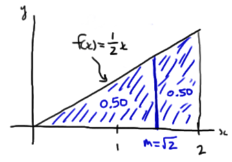
Throughout our discussion, and as the above illustration suggests, we'll assume that our random variable X is a continuous random variable with unknown median m. Upon taking a random sample \(X_1 , X_2 , \dots , X_n\), we'll be interested in testing whether the median m takes on a particular value \(m_0\). That is, we'll be interested in testing the null hypothesis:
\(H_0 \colon m = m_0 \)
against any of the possible alternative hypotheses:
\(H_A \colon m > m_0\) or \(H_A \colon m < m_0\) or \(H_A \colon m \ne m_0\)
Let's start by considering the quantity \(X_i - m_0\) for \(i = 1, 2, \dots , n\). If the null hypothesis is true, that is, \(m = m_0\), then we should expect about half of the \(x_i - m_0\) quantities obtained to be positive and half to be negative:
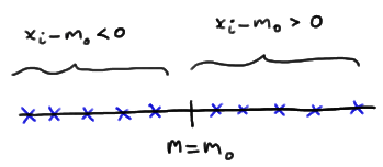
If instead, \(m > m_0\) , then we should expect more than half of the \(x_i - m_0\) quantities obtained to be positive and fewer than half to be negative:

Or, if instead, \(m < m_0\) , then we should expect fewer than half of the \(x_i - m_0\) quantities obtained to be positive and more than half to be negative:

This analysis of \(x_i - m_0\) under the three situations \(m = m_0\), \(m > m_0\) , and \(m < m_0\) suggests then that a reasonable test for testing the value of a median m should depend on \(X_i - m_0\) . That's exactly what the sign test for a median does. This is what we'll do:
- Calculate \(X_i - m_0\) for \(i = 1, 2, \dots , n\).
- Define N− = the number of negative signs obtained upon calculating \(X_i - m_0\) for \(i = 1, 2, \dots , n\).
- Define N+ = the number of positive signs obtained upon calculating \(X_i - m_0\) for \(i = 1, 2, \dots , n\).
Then, if the null hypothesis is true, that is, \(m = m_0\), then N− and N+ both follow a binomial distribution with parameters n and p = 1/2. That is:
\(N-\sim b\left(n, \frac{1}{2}\right)\) and \(N+\sim b\left(n, \frac{1}{2}\right)\)
Now, suppose we are interested in testing the null hypothesis \(H_0 \colon m = m_0\) against the alternative hypothesis \(H_A \colon m > m_0\). Then, if the alternative hypothesis were true, we should expect \(X_i - m_0\) to yield more positive (+) signs than would be expected if the null hypothesis were true:

In that case, we should reject the null hypothesis if n−, the observed number of negative signs, is too small, or alternatively, if the P-value as defined by:
\(P = P(N - \le n-)\)
is small, that is, less than or equal to \(\alpha\).
And, suppose we are interested in testing the null hypothesis \(H_0 \colon m = m_0\) against the alternative hypothesis \(H_A \colon m < m_0\). Then, if the alternative hypothesis were true, we should expect \(X_i - m_0\) to yield more negative (−) signs than would be expected if the null hypothesis were true:

In that case, we should reject the null hypothesis if n+, the observed number of positive signs, is too small, or alternatively, if the P-value as defined by:
\(P = P(N+ \le n+)\)
is small, that is, less than or equal to \(\alpha\).
Finally, if we are interested in testing the null hypothesis \(H_0 \colon m = m_0\) against the alternative hypothesis \(H_A \colon m \neq m_0\), it makes sense that we should reject the null hypothesis if we have too few negative signs or too few positive signs. Formally, we reject if \(n_{min}\), which is defined as the smaller of n− and n+, is too small. Alternatively, we reject if the P-value as defined by:
\(P = 2 \times P(N_{min} \le min(n-, n+))\)
is small, that is, less than or equal to \(\alpha\). Let's take a look at an example.
Example 20-1

Recent studies of the private practices of physicians who saw no Medicaid patients suggested that the median length of each patient visit was 22 minutes. It is believed that the median visit length in practices with a large Medicaid load is shorter than 22 minutes. A random sample of 20 visits in practices with a large Medicaid load yielded, in order, the following visit lengths:
9.4 13.4 15.6 16.2 16.4 16.8 18.1 18.7 18.9 19.1
 19.3 20.1 20.4 21.6 21.9 23.4 23.5 24.8 24.9 26.8
Based on these data, is there sufficient evidence to conclude that the median visit length in practices with a large Medicaid load is shorter than 22 minutes?
Answer
We are interested in testing the null hypothesis \(H_0 \colon m = 22\) against the alternative hypothesis \(H_A \colon m < 22\). To do so, we first calculate \(x_i − 22\), for \(i = 1, 2, \dots, 20\). Letting Minitab do the 20 subtractions for us, we get:
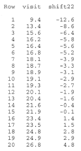
We can readily see that \(n+\), the observed number of positive signs, is 5. Therefore, we need to calculate how likely it would be to observe as few as 5 positive signs if the null hypothesis were true. Doing so, we get a P-value of 0.0207:

which is, of course, smaller than \(\alpha = 0.05\). The P-value tells us that it is not likely that we would observe so few positive signs if the null hypothesis were true. Therefore, we reject the null hypothesis in favor of the alternative hypothesis. There is sufficient evidence, at the 0.05 level, to conclude that the median visit length in practices with a large Medicaid load is shorter than 22 minutes.
Incidentally, we can use Minitab to conduct the sign test for us by selecting, under the Stat menu, Nonparametrics and then 1-Sample Sign. Doing so, we get:

Let's take a look at an example that illustrates how the sign test can even be applied to a situation in which the data are paired.
Example 20-2

A study is done to determine the effects of removing a renal blockage in patients whose renal function is impaired because of advanced metatstatic malignancy of nonurologic cause. The arterial blood pressure of a random sample of 10 patients is measured before and after surgery for treatment of the blockage yielded the following data:
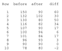
Based on the sign test, can we conclude that the surgery tends to lower arterial blood pressure?
Answer
We are interested in testing the null hypothesis \(H_0 \colon m_D = m_{B−A} = 0\) against the alternative hypothesis \(H_A \colon m_D = m_{B−A} > 0\). To do so, we just have to conduct a sign test while treating the differences as the data. If we look at the differences, we see that one of the differences is neither positive or negative, but rather zero. In this case, the standard procedure is to remove the observation that produces the zero, and reduce the number of observations by one. That is, we conduct the sign test using n = 9 rather than n = 10.
Now, n−, the observed number of negative signs, is 1, which yields a P-value of 0.0195:

The P-value is less than 0.05. Therefore, we can reject the null hypothesis. There is sufficient evidence, at the 0.05 level, to conclude that the surgery tends to lower arterial blood pressure.
Again, we can use Minitab to conduct the sign test for us. Doing so, we get:

Let's close up our discussion of the sign test by taking a note of the following:
- The sign test was presented here as a test for the median \(H_0 \colon m = m_0\), but if we were to make the additional assumption that the distribution of X is symmetric, then the sign test is also a valid test for the mean \(H_0 \colon \mu = \mu_0\).
- A primary advantage of the sign test is that by using only the signs of the \(X_i - m_0\) quantities, the test completely obliterates the negative effect of outliers.
- A primary disadvantage of the sign test is that by using only the signs of the \(X_i - m_0\) quantities, we potentially lose useful information about the magnitudes of the \(X_i - m_0\) quantities. For example, which data have more evidence against the null hypothesis \(H_0 \colon m = m_0\)? (1, 1, −1) versus (5, 6, −1)? Or (1, 1, −1) versus (10000, 6, −1)?
That last point suggests that we might want to also consider a test that takes into account the magntitudes of the \(X_i - m_0\) quantities. That's exactly what the Wilcoxon signed rank test does. Let's go check it out.
20.2 - The Wilcoxon Signed Rank Test for a Median
20.2 - The Wilcoxon Signed Rank Test for a MedianDeveloped in 1945 by the statistician Frank Wilcoxon, the signed rank test was one of the first "nonparametric" procedures developed. It is considered a nonparametric procedure, because we make only two simple assumptions about the underlying distribution of the data, namely that:
- The random variable X is continuous
- The probablility density function of X is symmetric
Then, upon taking a random sample \(X_1 , X_2 , \dots , X_n\), we are interested in testing the null hypothesis:
\(H_0 : m=m_0\)
against any of the possible alternative hypotheses:
\(H_A : m > m_0\) or \(H_A : m < m_0\) or \(H_A : m \ne m_0\)
As we often do, let's motivate the procedure by way of example.
Example 20-3

Let \(X_i\) denote the length, in centimeters, of a randomly selected pygmy sunfish, \(i = 1, 2, \dots 10\). If we obtain the following data set:
5.0 3.9 5.2 5.5 2.8 6.1 6.4 2.6 1.7 4.3
can we conclude that the median length of pygmy sunfish differs significantly from 3.7 centimeters?
Answer
We are interested in testing the null hypothesis \(H_0: m = 3.7\) against the alternative hypothesis \(H_A: m ≠ 3.7\). In general, the Wilcoxon signed rank test procedure requires five steps. We'll introduce each of the steps as we apply them to the data in this example.
- Step 1
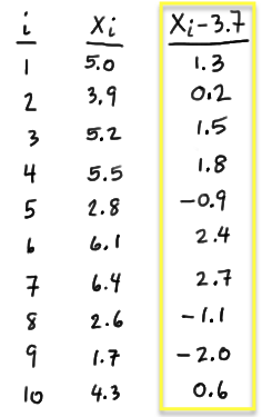
In general, calculate \(X_i − m_0\) for \(i = 1, 2, \dots , n\). In this case, we have to calculate \(X_i − 3.7\) for \(i = 1, 2, \dots , 10\):
- Step 2
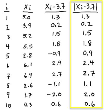
In general, calculate the absolute value of \(X_i − m_0\), that is, \(|X_i − m_0|\) for \(i = 1, 2, \dots , n\). In this case, we have to calculate \(|X_i − 3.7|\) for \(i = 1, 2, \dots , 10\):
- Step 3
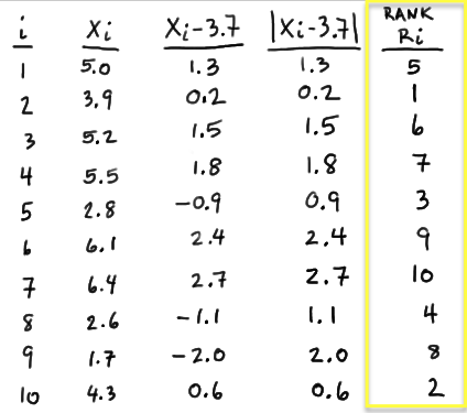
Determine the rank \(R_i, i = 1, 2,\dots , n\) of the absolute values (in ascending order) according to their magnitude. In this case, the value of 0.2 is the smallest, so it gets rank 1. The value of 0.6 is the next smallest, so it gets rank 2. We continue ranking the data in this way until we have assigned a rank to each of the data values:
- Step 4
Determine the value of W, the Wilcoxon signed-rank test statistic:
\( W=\sum_{i=1}^{n}Z_i R_i\)
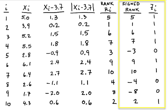
where \(Z_i\) is an indicator variable with \(Z_i = 0\) if \(X_i − m_0\) is negative and \(Z_i = 1\) if \(X_i − m_0\) is positive. That is, with \(Z_i\) defined as such, W is then the sum of the positive signed ranks. In this case, because the first observation yields a positive \(X_1 − 3.7\), namely 1.3, \(Z_1 = 1\). Because the fifth observation yields a negative \(X_5 − 3.7\), namely −0.9, \(Z_5 = 0\). Determining \(Z_i\) as such for \(i = 1, 2, \dots , 10\), we get:
And, therefore W equals 40:
\( W=(1)(5)+(1)(1)+ ... +(0)(-8)+(1)(2) =5+1+6+7+9+10+2=40\)
- Step 5
Determine if the observed value of W is extreme in light of the assumed value of the median under the null hypothesis. That is, calculate the P-value associated with W, and make a decision about whether to reject or not to reject. Whoa, nellie! We're going to have to take a break from this example before we can finish, as we first have to learn something about the distribution of W.
The Distribution of W
As is always the case, in order to find the distribution of the discrete random variable W, we need:
- To find the range of possible values of W, that is, we need to specify the support of W
- To determine the probability that W takes on each of the values in the support
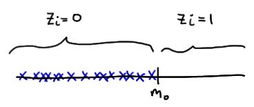
Let's tackle the support of W first. Well, the smallest that \(W=\sum_{i=1}^{n}Z_i R_i\) could be is 0. That would happen if each observation \(X_i\) fell below the value of the median \(m_0\) specified in the null hypothesis, thereby causing \(Z_i = 0\), for \(i = 1, 2, \dots , n\):
The largest that \(W=\sum_{i=1}^{n}Z_i R_i\) could be is \(\dfrac{n(n+1)}{2}\). That would happen if each observation fell above the value of the median \(m_0\) specified in the null hypothesis, thereby causing \(z_i = 1\), for \(i = 1, 2, \dots , n\):
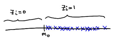
and therefore W reduces to the sum of the integers from 1 to n:
\(W=\sum_{i=1}^{n}Z_i R_i=\sum_{i=1}^{n}=\dfrac{n(n+1)}{2}\)
So, in summary, W is a discrete random variable whose support ranges between 0 and n(n+1)/2.
Now, if we have a small sample size n, such as we do in the above example, we could use the exact probability distribution of W to calculate the P-values for our hypothesis tests. Errr.... first we have to determine the exact probability distribution of W. Doing so is very doable. It just takes some thinking and perhaps a bit of tedious work. Let's make our discussion concrete by considering a very small sample size, n = 3, say. In that case, the possible values of W are the integers 0, 1, 2, 3, 4, 5, 6. Now, each of the three data points would be assigned a rank \(R_i\) of either 1, 2, or 3, and depending on whether the data point fell above or below the hypothesized median \(m_0\), each of the three possible ranks 1, 2, or 3 would remain either a positive signed rank or become a negative signed rank. In this case, because we are considering such a small sample size, we can easily enumerate each of the possible outcomes, as well as sum W of the positive ranks to see how each arrangement results in one of the possible values of W:

There we have it. We're just about done with finding the exact probability distribution of W when n = 3. All we have to do is recognize that under the null hypothesis, each of the above eight arrangements (columns) is equally likely. Therefore, we can use the classical approach to assigning the probabilities. That is:
- P(W = 0) = 1/8, because there is only one way that W = 0
- P(W = 1) = 1/8, because there is only one way that W = 1
- P(W = 2) = 1/8, because there is only one way that W = 2
- P(W = 3) = 2/8, because there are two ways that W = 3
- P(W = 4) = 1/8, because there is only one way that W = 4
- P(W = 5) = 1/8, because there is only one way that W = 5
- P(W = 6) = 1/8, because there is only one way that W = 6
And, just to make sure that we haven't made an error in our calculations, we can verify that the sum of the probabilities over the support 0, 1, ..., 6 is indeed 1/8 + 1/8 + ... + 1/8 = 1.
Hmmm. That was easy enough. Let's do the same thing for a sample size of n = 4. Well, in that case, the possible values of W are the integers 0, 1, 2, ..., 10. Now, each of the four data points would be assigned a rank \(R_i\) of either 1, 2, 3, or 4, and depending on whether the data point fell above or below the hypothesized median \(m_0\), each of the three possible ranks 1, 2, 3, or 4 would remain either a positive signed rank or become a negative signed rank. Again, because we are considering such a small sample size, we can easily enumerate each of the possible outcomes, as well as sum W of the positive ranks to see how each arrangement results in one of the possible values of W:

Again, under the null hypothesis, each of the above 16 arrangements is equally likely, so we can use the classical approach to assigning the probabilities:
- P(W = 0) = 1/16, because there is only one way that W = 0
- P(W = 1) = 1/16, because there is only one way that W = 1
- P(W = 2) = 1/16, because there is only one way that W = 2
- P(W = 3) = 2/16, because there are two ways that W = 3
- and so on...
- P(W = 9) = 1/16, because there is only one way that W = 9
- P(W = 10) = 1/16, because there is only one way that W = 10
Do you want to do the calculation for the case where n = 5? Here's what the enumeration of possible outcomes looks like:
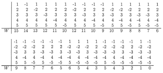
After having worked through finding the exact probability distribution of W for the cases where n = 3, 4, and 5, we should be able to make some generalizations. First, note that, in general, there are \(2^n\) total number of ways to make signed rank sums, and therefore the probability that W takes on a particular value w is:
\(P(W=w)=f(w)=\dfrac{c(w)}{2^n}\)
where c(w) = the number of possible ways to assign a + or a − to the first n integers so that \(\sum_{i=1}^{n}Z_i R_i=w\).
Okay, now that we have the general idea of how to determine the exact probability distribution of W, we can breathe a sigh of relief when it comes to actually analyzing a set of data. That's because someone else has done the dirty work for us for sample sizes n = 3, 4, ..., 12, and published the relevant results in a statistical table of W. (Our textbook authors chose not to include such a table in our textbook.) By relevant, I mean the probabilities in the "tails" of the distribution of W. After all, that's what P-values generally are, that is, probabilities in the tails of the distribution under the null hypothesis.
As the table of W suggests, our determination of the probability distribution of W when n = 4 agrees with the results published in the table:

because both we and the table claim that:
\(P(W \le 0)=P(W \ge 10)=0.062\)
and:
\(P(W \le 1)=P(W =0)+P(W =1)=0.062+0.062=0.125\)
\(P(W \ge 9)=P(W =9)+P(W =10)=0.062+0.062=0.125\)
Okay, it should be pretty obvious that working with the exact distribution of W is going to be pretty limiting when it comes to large sample sizes. In that case, we do what we typically do when we have large sample sizes, namely use an approximate distribution of W.
When the null hypothesis is true, for large n:
\(W'={\sum_{i=1}^{n}Z_i R_i - \dfrac{n(n+1)}{4} \over \sqrt{\frac{n(n+1)(2n+1)}{24}}}\)
follows an approximate standard normal distribution N(0, 1).
Proof
Because the Central Limit Theorem is at work here, the approximate standard normal distribution part of the theorem is trivial. Our proof therefore reduces to showing that the mean and variance of W are:
\(E(W)=\dfrac{n(n+1)}{4}\) and \(Var(W)=\dfrac{n(n+1)(2n+1)}{24}\)
respectively. To find E(W) and Var(W), note that \(W=\sum_{i=1}^{n}Z_i R_i\) has the same distribution of \(U=\sum_{i=1}^{n}U_i\) where:
- \(U_i\) with probability ½
- \(U_i = i\) with probability ½
In case that claim was less than obvious, consider this intuitive, hand-waving kind of argument:
- W and U are both sums of a subset of the numbers 1, 2, ..., n
- Under symmetry, an equally likely chance of getting assigned either a + or a − is equivalent to having an equally likely chance of being included in the sum or not.
At any rate, we therefore have:
\(E(W)=E(U)=\sum_{i=1}^{n}E(U_i)=\sum_{i=1}^{n}\left[0\left(\dfrac{1}{2}\right)+i\left(\dfrac{1}{2}\right) \right]=\dfrac{1}{2}\sum_{i=1}^{n}i=\dfrac{1}{2}\times\frac{n(n+1)}{2}=\dfrac{n(n+1)}{4} \)
and:
\(Var(W) =Var(U)=\sum_{i=1}^{n}Var(U_i)\)
because the Ui's are independent under the null hypothesis. Now:
\(Var(U_i) = E(U_{i}^{2})-E(U_i)^2 = \left[0^2\left(\dfrac{1}{2}\right)+i^2\left(\dfrac{1}{2}\right) \right]-\left(\dfrac{i}{2}\right)^2 = \dfrac{i^2}{2}-\dfrac{i^2}{4} = \dfrac{i^2}{4}\)
and therefore:
\(Var(W)=\sum_{i=1}^{n}Var(U_i)=\sum_{i=1}^{n}\dfrac{i^2}{4}=\dfrac{1}{4}\sum_{i=1}^{n}i^2=\dfrac{1}{4}\times\dfrac{n(n+1)(2n+1)}{6} \)
Therefore, in summary, under the null hypothesis, we have that:
\(W'=\dfrac{\sum_{i=1}^{n}Z_i R_i - \dfrac{n(n+1)}{4}}{\sqrt{\frac{n(n+1)(2n+1)}{24}}} \)
follows an approximate standard normal distribution as was to be proved.
Let's return to our example now to complete our work.
Example 20-3 (continued)

Let \(X_i\) denote the length of a randomly selected pygmy sunfish, \(i = 1, 2, \dots 10\). If we obtain the following data set:
5.0 3.9 5.2 5.5 2.8 6.1 6.4 2.6 1.7 4.3
can we conclude that the median length of pygmy sunfish differs significantly from 3.7 centimeters?
Answer
Recall that we are interested in testing the null hypothesis \(H_0 \colon m = 3.7\) against the alternative hypothesis \(H_A \colon m ≠ 3.7\). The last time we worked on this example, we got as far as determining that W = 40 for the given data set. Now, we just have to use what we know about the distribution of W to complete our hypothesis test. Well, in this case, with n = 10, our sample size is fairly small so we can use the exact distribution of W. The upper and lower percentiles of the Wilcoxon signed rank statistic when n = 10 are:
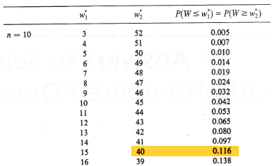
Therefore, our P-value is 2 × 0.116 = 0.232. Because our P-value is large, we cannot reject the null hypothesis. There is insufficient evidence at the 0.05 level to conclude that the median length of pygmy sunfish differs significantly from 3.7 centimeters.
Notes
A couple of notes are worth mentioning before we take a look at another example:
- Our textbook authors define \(W=\sum_{i=1}^{n}R_i\) as the sum of all of the ranks, as opposed to just the sum of the positive ranks. That is perfectly fine, but not the most typical way of defining W.
- W is based on the ranks of the deviations from the hypothesized median \(m_0\), not on the deviations themselves. In the above example, W = 40 even if x7 = 6.4 or 10000 (now that's a pretty strange sunfish) because its rank would be unchanged. It is in this sense that W protects against the effect of outliers.
Now for that last example.
Example 20-4

The median age of the onset of diabetes is thought to be 45 years. The ages at onset of a random sample of 30 people with diabetes are:
35.5 44.5 39.8 33.3 51.4 51.3 30.5 48.9 42.1 40.3
46.8 38.0 40.1 36.8 39.3 65.4 42.6 42.8 59.8 52.4
26.2 60.9 45.6 27.1 47.3 36.6 55.6 45.1 52.2 43.5
Assuming the distribution of the age of the onset of diabetes is symmetric, is there evidence to conclude that the median age of the onset of diabetes differs significantly from 45 years?
Answer
We are interested in testing the null hypothesis \(H_0 \colon m = 45\) against the alternative hypothesis \(H_A \colon m ≠ 45\). We can use Minitab's calculator and statistical functions to do the dirty work for us:
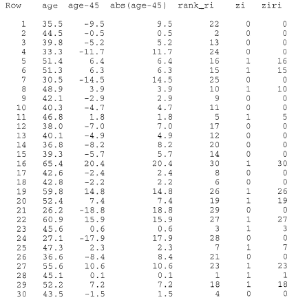
Then, summing the last column, we get:

Because we have a large sample (n = 30), we can use the normal approximation to the distribution of W. In this case, our P-value is defined as two times the probability that W ≤ 200. Therefore, using a half-unit correction for continuity, our transformed signed rank statistic is:
\(W'=\dfrac{200.5 - \left(\frac{30(31)}{4}\right)}{\sqrt{\frac{30(31)(61)}{24}}}=-0.6581 \)
Therefore, upon using a normal probability calculator (or table), we get that our P-value is:
\(P \approx 2 \times P(W' < -0.66)=2(0.2546) \approx 0.51 \)
Because our P-value is large, we cannot reject the null hypothesis. There is insufficient evidence at the 0.05 level to conclude that the median age of the onset of diabetes differs significantly from 45 years.
By the way, we can even be lazier and let Minitab do all of the calculation work for us. Under the Stat menu, if we select Nonparametrics, and then 1-Sample Wilcoxon, we get:

20.3 - Tied Observations
20.3 - Tied ObservationsAll of our examples thus far have involved unique observations. That is, there were no tied observations. Dealing with ties is simple enough. If the absolute values of the differences from \(m_0\) of two or more observations are equal, each observation is assigned the average of the corresponding ranks. The change this causes in the distribution of W is not all that great.
Example 20-5

Dental researchers have developed a new material for preventing cavities, a plastic sealant that is applied to the chewing surfaces of teeth. To determine whether the sealant is effective, it was applied to half of the teeth of each of 12 school-aged children. After two years, the number of cavities in the sealant-coated teeth and in the uncoated teeth were counted, resulting in the following data:
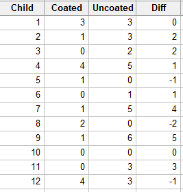
Is there sufficient evidence to indicate that sealant-coated teeth are less prone to cavities than are untreated teeth? (From Wackerly, Mendenhall, & Scheaffer, seventh edition.)
Answer
Let X denote the number of cavities in the uncoated teeth, and Y denote the number of cavities in the coated teeth. Then, we're interested in analyzing the differences D = X−Y. Specifically, if m is the median of the differences D = X−Y, then we're interested in testing the null hypothesis \(H_0 \colon m = 0\) against the alternative hypothesis \(H_A \colon m > 0\). Analyzing the differences, we see that two of the differences are 0, and so we eliminate them from the analysis:
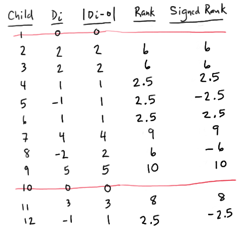
Assigning ranks to the remaining 10 data points, we see that we have two sets of tied observations. Because there are four 1s, we assign them the average of the ranks 1, 2, 3, and 4, that is, 2.5. Having used up the ranks 1, 2, 3, and 4, because 2 is the next set of tied observations, the three 2s are assigned the average of the ranks 5, 6, and 7, that is, 6. Having used up the ranks from 1 to 7, the remaining three unique observations get assigned the ranks 8, 9, and 10. When all is said and done, W, the sum of the positive ranks is:
W = 6 + 6 + 2.5 + 2.5 + 9 + 10 + 8 = 44
The statistical table for W:
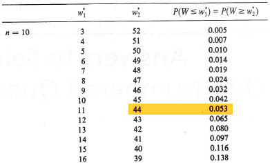
tells us that the P-value is P(W ≥ 44) = 0.053. There is just barely not enough evidence, at the 0.05 level, to reject the null hypothesis. (I do imagine that a larger sample may have lead to a significant result.)
Alternatively, we could have completely ignored the condition of the data, that is, whether or not there were ties, and put the data into the black box of Minitab, getting:
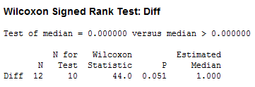
We see that our analysis is consistent with the results from Minitab, namely 10 data points yield a Wilcoxon statistic of 44.0 and a P-value of 0.051 (round-off error).