Answer

As reported, the data are ordered, therefore the order statistics are \(y_1 = 0, y_2 = 1, y_3 = 2, y_4 = 2, y_5 = 4, y_6 = 6, y_7 = 6\) and \(y_8 = 7\). Therefore, using the definition of the empirical distribution function, we have:

\(F_n(x)=0 \text{ for } x < 0\)

and:

\(F_n(x)=\frac{1}{8} \text{ for } 0 \le x < 1\) and \(F_n(x)=\frac{2}{8} \text{ for } 1 \le x < 2\)

Now, noting that there are two 2s, we need to jump 2/8 at x = 2:

\(F_n(x)=\frac{2}{8}+\frac{2}{8}=\frac{4}{8} \text{ for } 2 \le x < 4\)

Then:

\(F_n(x)=\frac{5}{8} \text{ for } 4 \le x < 6\)

Again, noting that there are two 6s, we need to jump 2/8 at x = 6:

\(F_n(x)=\frac{5}{8}+\frac{2}{8}=\frac{7}{8} \text{ for } 6 \le x < 7\)

And, finally:

\(F_n(x)=\frac{7}{8}+\frac{1}{8}=\frac{8}{8}=1 \text{ for } x \ge 7\)

Plotting the function, it should look something like this then:

Answer

The probability density function of a Uniform(0, 2) random variable X, say, is:

\( f(x)=\frac{1}{2}\)

for 0 < x < 2. Therefore, the probability that X is less than or equal to x is:

\(P(X \le x) =\int_{0}^{x}\frac{1}{2}dt=\frac{1}{2}x\)

for 0 < x < 2, and we are interested in testing:

• the null hypothesis \(H_0 : F(x)=F_0(x)\) against
• the alternative hypothesis \(H_A : F(x) \ne F_0(x)\)

where F(x) is the (unknown) cdf from which our data were sampled, and

Now, in working towards calculating \(d_n\), we first need to order the eight data points so that \(y_1\le \cdots\le y_8\). The table below provides all the necessary values for finding the KS test statistic. Note that the empirical cdf satisfies \(F_n(y_k)=k/8\), for \(k=0,1,\ldots,8\).

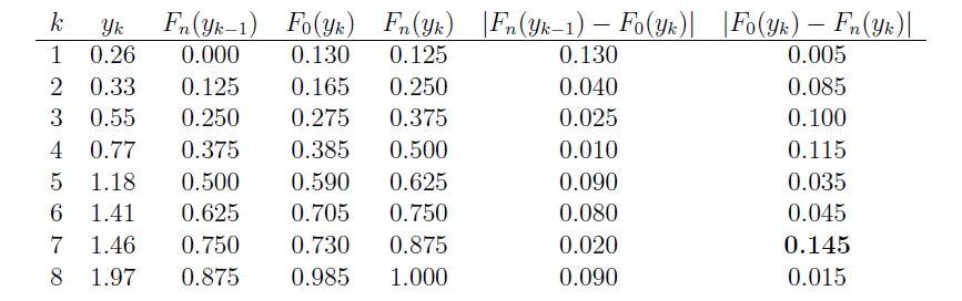
The last two columns represent all the differences we need to check. The largest of these is \(d_8=0.145\). From the table below with \(\alpha=0.05\), the critical value is \(0.46\). So, we can not reject the claim that the data were sampled from Uniform(0,2).

Answer

We are interested in testing the null hypothesis, \(H_0:\) \(X\) is normally distributed with mean 120 and standard deviation 10, against the alternative hypothesis, \(H_A\): \(X\) is not normally distributed with mean 120 and standard deviation 10. Now, in working towards calculating \(d_n\), we again first need to order the ten data points so that \(y_1=105\), \(y_2=108\), etc. Then, we need to calculate the value of the hypothesized distribution function \(F_0(y_k)\) at each of the values of \(y_k\). The standard normal table can help us do this. The probability that \(X\) is less than or equal to 105, for example, equals the probability that \(Z\) is less than or equal to \(-1.5\):

\(F_0(y_1)=P(X\le105)=P\left(Z\le{105-120\over10}\right)=P(Z\le-1.5)=.0668.\)

The table below summarizes the relevant quantities for finding the KS test statistic. Note that the empirical cdf satisfies \(F_n(y_k)=k/10\), except at \(k=5\) because of the tie: \(y_5=y_6=113\).

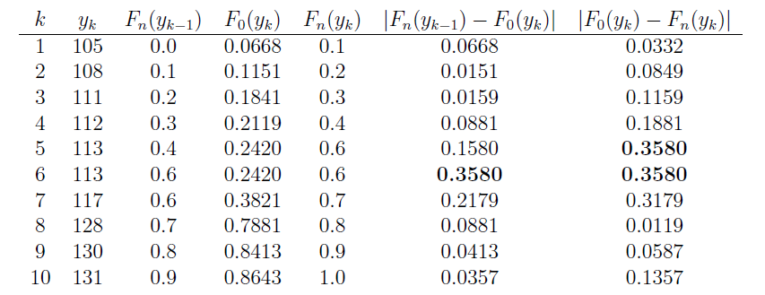
The last two columns represent all the differences we need to check. The largest of these is 0.3580. From the table below with \(\alpha=0.10\), the critical value is 0.37. Because \(d_{10} = 0.358\), which is just barely less than 0.37, we do not reject the null hypothesis at the 0.10 level. There is not enough evidence at the 0.10 level to reject the assumption that the data were randomly sampled from a normal distribution with mean 120 and standard deviation 10.

Answer

As before, we start by ordering the x values. The formulas for the lower and upper confidence limits tell us that we need to know d and \(F_n (x)\) for each of the 10 data points. Because the \(\alpha\)-level is 0.05 and the sample size n is 10, the table of Kolmogorv-Smirnov Acceptance Limits in the back of our text book, that is, Table VIII, tells us that \(d = 0.41\). We already calculated \(F_n (x)\) in the previous example.

Now, in calculating the lower limit, \(F_L(x) = F_n (x) − d = F_n (x)−0.41\), we see that the lower limit would be negative for the first four data points:

0.1−0.41 = −0.31 and 0.2−0.41 = −0.21 and 0.3−0.41 = −0.11 and 0.4−0.41 = −0.01

Therefore, we assign the first four data points a lower limit of 0, and then just calculate the remaining lower limit values. Similarly, in calculating the upper limit, \(F_U (x) = F_n (x) + d = F_n (x) + 0.41\), we see that the upper limit would be greater than 1 for the last six data points:

0.6+0.41 = 1.01 and 0.7+0.41 = 1.11 and 0.8+0.41 = 1.21 and 0.9+0.41 = 1.31 and 1.0+0.41 = 1.41

Therefore, we assign the last six data points an upper limit of 1, and then just calculate the remaining upper limit values. To summarize,

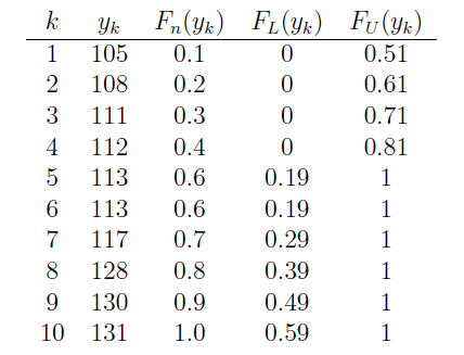
The last two columns together give us the 95% confidence band for the unknown cumulative distribution function \(F(x)\).