Answer

If the null parameter space is \(\Omega = {\mu: \mu = 3}\), then the alternative parameter space is everything that is in \(\Omega = {\mu: −∞ < \mu < ∞}\) that is not in \(\Omega\). That is, the alternative parameter space is \(\Omega ' = {\mu: \mu ≠ 3}\). And, so the alternative hypothesis is:

\(H_A : \mu \ne 3\)

In this case, we'd be interested in deriving a two-tailed test.

Answer

If the alternative parameter space is (\omega ' = {\mu: \mu > 3}\), then the null parameter space is \(\omega = {\mu: \mu ≤ 3}\). And, so the null hypothesis is:

\(H_0 : \mu \le 3\)

Now, the reality is that some authors do specify the null hypothesis as such, even when they mean \(H_0: \mu = 3\). Ours don't, and so we won't. (That's why I put that "technically" in parentheses up above.) At any rate, in this case, we'd be interested in deriving a one-tailed test.

Answer

Because we are interested in testing the null hypothesis \(H_0: \mu = 10\) against the alternative hypothesis \(H_A: \mu ≠ 10\) for a normal mean, our total parameter space is:

\(\Omega =\left \{\mu : -\infty < \mu < \infty \right \}\)

and our null parameter space is:

\(\omega = \left \{10\right \}\)

Now, to find the likelihood ratio, as defined above, we first need to find \(L(\hat{\omega})\). Well, when the null hypothesis \(H_0: \mu = 10\) is true, the mean \(\mu\) can take on only one value, namely, \(\mu = 10\). Therefore:

\(L(\hat{\omega}) = L(10)\)

We also need to find \(L(\hat{\Omega})\) in order to define the likelihood ratio. To find it, we must find the value of \(\mu\) that maximizes \(L(\mu)\). Well, we did that back when we studied maximum likelihood as a method of estimation. We showed that \(\hat{\mu} = \bar{x}\) is the maximum likelihood estimate of \(\mu\). Therefore:

\(L(\hat{\Omega}) = L(\bar{x})\)

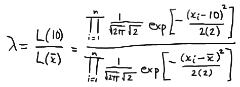
Now, putting it all together to form the likelihood ratio, we get:

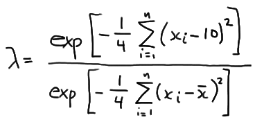
which simplifies to:

Now, let's step aside for a minute and focus just on the summation in the numerator. If we "add 0" in a special way to the quantity in parentheses:

we can show that the summation can be written as:

\(\sum_{i=1}^{n}(x_i - 10)^2 = \sum_{i=1}^{n}(x_i - \bar{x})^2 + n(\bar{x} -10)^2 \)

Therefore, the likelihood ratio becomes:

which greatly simplifies to:

\(\lambda = exp \left [-\dfrac{n}{4}(\bar{x}-10)^2 \right ]\)

Now, the likelihood ratio test tells us to reject the null hypothesis when the likelihood ratio \(\lambda\) is small, that is, when:

\(\lambda = exp\left[-\dfrac{n}{4}(\bar{x}-10)^2 \right] \le k\)

where k is chosen to ensure that, in this case, \(\alpha = 0.05\). Well, by taking the natural log of both sides of the inequality, we can show that \(\lambda ≤ k\) is equivalent to:

\( -\dfrac{n}{4}(\bar{x}-10)^2 \le \text{ln} k \)

which, by multiplying through by −4/n, is equivalent to:

\((\bar{x}-10)^2 \ge -\dfrac{4}{n} \text{ln} k \)

which is equivalent to:

\(\dfrac{|\bar{X}-10|}{\sigma / \sqrt{n}} \ge \dfrac{\sqrt{-(4/n)\text{ln} k}}{\sigma / \sqrt{n}} =k* \)

Aha! We should recognize that quantity on the left-side of the inequality! We know that:

\(Z = \dfrac{\bar{X}-10}{\sigma / \sqrt{n}} \)

follows a standard normal distribution when \(H_0: \mu = 10\). Therefore we can determine the appropriate \(k^*\) by using the standard normal table. We have shown that the likelihood ratio test tells us to reject the null hypothesis \(H_0: \mu = 10\) in favor of the alternative hypothesis \(H_A: \mu ≠ 10\) for all sample means for which the following holds:

\(\dfrac{|\bar{X}-10|}{ \sqrt{2} / \sqrt{n}} \ge z_{0.025} = 1.96 \)

Doing so will ensure that our probability of committing a Type I error is set to \(\alpha = 0.05\), as desired.

Answer

Our unrestricted parameter space is:

\( \Omega = \left\{ (\mu, \sigma^2) : -\infty < \mu < \infty, 0 < \sigma^2 < \infty \right\} \)

Under the null hypothesis, the mean \(\mu\) is the only parameter that is restricted. Therefore, our parameter space under the null hypothesis is:

\( \omega = \left\{(\mu, \sigma^2) : \mu =\mu_0, 0 < \sigma^2 < \infty \right\}\)

Now, first consider the case where the mean and variance are unrestricted. We showed back when we studied maximum likelihood estimation that the maximum likelihood estimates of \(\mu\) and \(\sigma^2\) are, respectively:

\(\hat{\mu} = \bar{x} \text{ and } \hat{\sigma}^2 = \dfrac{1}{n}\sum_{i=1}^{n}(x_i - \bar{x})^2 \)

Therefore, the maximum of the likelihood function for the unrestricted parameter space is:

which simplifies to:

\( L(\hat{\Omega})= \left[\dfrac{ne^{-1}}{2\pi \Sigma (x_i - \bar{x})^2} \right]^{n/2} \)

Now, under the null parameter space, the maximum likelihood estimates of \(\mu\) and \(\sigma^2\) are, respectively:

\( \hat{\mu} = \mu_0 \text{ and } \hat{\sigma}^2 = \dfrac{1}{n}\sum_{i=1}^{n}(x_i - \mu_0)^2 \)

Therefore, the likelihood under the null hypothesis is:

which simplifies to:

\( L(\hat{\omega})= \left[\dfrac{ne^{-1}}{2\pi \Sigma (x_i - \mu_0)^2} \right]^{n/2} \)

And now taking the ratio of the two likelihoods, we get:

which reduces to:

\( \lambda = \left[ \dfrac{\sum_{i=1}^{n}(x_i - \bar{x})^2}{\sum_{i=1}^{n}(x_i - \mu_0)^2} \right] ^{n/2}\)

Focusing only on the denominator for a minute, let's do that trick again of "adding 0" in just the right away. Adding 0 to the quantity in the parentheses, we get:

which simplifies to:

\( \sum_{i=1}^{n}(x_i - \mu_0)^2 = \sum_{i=1}^{n}(x_i - \bar{x})^2 +n(\bar{x} - \mu_0)^2 \)

Then, our likelihood ratio \(\lambda\) becomes:

\( \lambda = \left[ \dfrac{\sum_{i=1}^{n}(x_i - \bar{x})^2}{\sum_{i=1}^{n}(x_i - \mu_0)^2} \right] ^{n/2} = \left[ \dfrac{\sum_{i=1}^{n}(x_i - \bar{x})^2}{ \sum_{i=1}^{n}(x_i - \bar{x})^2 +n(\bar{x} - \mu_0)^2} \right] ^{n/2} \)

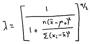
which, upon dividing through numerator and denominator by \( \sum_{i=1}^{n}(x_i - \bar{x})^2 \) simplifies to:

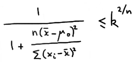
Therefore, the likelihood ratio test's critical region, which is given by the inequality \(\lambda ≤ k\), is equivalent to:

which with some minor algebraic manipulation can be shown to be equivalent to:

So, in a nutshell, we've shown that the likelihood ratio test tells us that for this situation we should reject the null hypothesis \(H_0: \mu= \mu_0\) in favor of the alternative hypothesis \(H_A: \mu ≠ \mu_0\) if:

\( \dfrac{(\bar{x}-\mu_0)^2 }{s^2 / n} \ge k^{*} \)

Well, okay, so I started out this page claiming that the t-test for a mean \(\mu\) is the likelihood ratio test. Is it? Well, the above critical region is equivalent to rejecting the null hypothesis if:

\( \dfrac{|\bar{x}-\mu_0| }{s / \sqrt{n}} \ge k^{**} \)

Does that look familiar? We previously learned that if \(X_1, X_2, \dots, X_n\) are normally distributed with mean \(\mu\) and variance \(\sigma^2\), then:

\( T = \dfrac{\bar{X}-\mu}{S / \sqrt{n}} \)

follows a T distribution with n − 1 degrees of freedom. So, this tells us that we should use the T distribution to choose \(k^{**}\). That is, set:

\(k^{**} = t_{\alpha /2, n-1}\)

and we have our size \(\alpha\) t-test that ensures the probability of committing a Type I error is \(\alpha\).