16.3 - Unspecified Probabilities
16.3 - Unspecified ProbabilitiesFor the two examples that we've thus far considered, the probabilities were pre-specified. For the first example, we were interested in seeing if the data fit a probability model in which there was a 0.60 probability that a randomly selected Penn State student was female. In the second example, we were interested in seeing if the data fit a probability model in which the probabilities of selecting a brown, yellow, orange, green, and coffee-colored candy was 0.4, 0.2, 0.2, 0.1, and 0.1, respectively. That is, we were interested in testing specific probabilities:
\(H_0 : p_{B}=0.40,p_{Y}=0.20,p_{O}=0.20,p_{G}=0.10,p_{C}=0.10 \)
Someone might be also interested in testing whether a data set follows a specific probability distribution, such as:
\(H_0 : X \sim b(n, 1/2)\)
What if the probabilities aren't pre-specified though? That is, suppose someone is interested in testing whether a random variable is binomial, but with an unspecified probability of success:
\(H_0 : X \sim b(n, p)\)
Can we still use the chi-square goodness-of-fit statistic? The short answer is yes... with just a minor modification.
Example 16-4
Let X denote the number of heads when four dimes are tossed at random. One hundred repetitions of this experiment resulted in 0, 1, 2, 3, and 4 heads being observed on 8, 17, 41, 30, and 4 trials, respectively. Under the assumption that the four dimes are independent, and the probability of getting a head on each coin is p, the random variable X is b(4, p). In light of the observed data, is b(4, p) a reasonable model for the distribution of X?
Answer
In order to use the chi-square statistic to test the data, we need to be able to determine the observed and expected number of trials in which we'd get 0, 1, 2, 3, and 4 heads. The observed part is easy... we know those:
| X | 0 | 1 | 2 | 3 | 4 |
|---|---|---|---|---|---|
| Observed | 8 | 17 | 41 | 30 | 4 |
| Expected |
It's the expected numbers that are a problem. If the probability p of getting ahead were specified, we'd be able to calculate the expected numbers. Suppose, for example, that p = 1/2. Then, the probability of getting zero heads in four dimes is:
\(P(X=0)=\binom{4}{0}\left(\dfrac{1}{2}\right)^0\left(\dfrac{1}{2}\right)^4=0.0625 \)
and therefore the expected number of trials resulting in 0 heads is 100 × 0.0625 = 6.25. We could make similar calculations for the case of 1, 2, 3, and 4 heads, and we would be well on our way to using the chi-square statistic:
\(Q_4=\sum_{i=0}^{4}\dfrac{(Obs_i-Exp_i)^2}{Exp_i} \)
and comparing it to a chi-square distribution with 5−1 = 4 degrees of freedom. But, we don't know p, as it is unspecified! What do you think the logical thing would be to do in this case? Sure... we'd probably want to estimate p. But then that begs the question... what should we use as an estimate of p?
One way of estimating p would be to minimize the chi-square statistic \(Q_4\) with respect to p, yielding an estimator \(\tilde{p}\). This \(\tilde{p}\) estimator is called, perhaps not surprisingly, a minimum chi-square estimator of p. If \(\tilde{p}\) is used in calculating the expected numbers that appear in \(Q_4\), it can be shown (not easily, and therefore we won't!) that \(Q_4\) still has an approximate chi-square distribution but with only 4−1 = 3 degrees of freedom. The number of degrees of freedom of the approximating chi-square distribution is reduced by one because we have to estimate one parameter in order to calculate the chi-square statistic. In general, the number of degrees of freedom of the approximating chi-square distribution is reduced by d, the number of parameters estimated. If we estimate two parameters, we reduce the degrees of freedom by two. And so on.
This all seems simple enough. There's just one problem... it is usually very difficult to find minimum chi-square estimators. So what to do? Well, most statisticians just use some other reasonable method of estimating the unspecified parameters, such as maximum likelihood estimation. The good news is that the chi-square statistic testing method still works well. (It should be noted, however, that the approach does provide a slightly larger probability of rejecting the null hypothesis than would the approach based purely on the minimized chi-square.)
Let's summarize
Chi-square method when parameters are unspecified. If you are interested in testing whether a data set fits a probability model with d parameters left unspecified:
- Estimate the d parameters using the maximum likelihood method (or another reasonable method).
- Calculate the chi-square statistic \(Q_{k−1}\) using the obtained estimates.
- Compare the chi-square statistic to a chi-square distribution with (k−1)−d degrees of freedom.
Example 16-5
Let X denote the number of heads when four dimes are tossed at random. One hundred repetitions of this experiment resulted in 0, 1, 2, 3, and 4 heads being observed on 8, 17, 41, 30, and 4 trials, respectively. Under the assumption that the four dimes are independent, and the probability of getting a head on each coin is p, the random variable X is b(4, p). In light of the observed data, is b(4, p) a reasonable model for the distribution of X?
Answer
Given that four dimes are tossed 100 times, we have 400 coin tosses resulting in 205 heads for an estimated probability of success of 0.5125:
\(\hat{p}=\dfrac{0(8)+1(17)+2(41)+3(30)+4(4)}{400}=\dfrac{205}{400}=0.5125 \)
Using 0.5125 as the estimate of p, we can use the binomial p.m.f. (or Minitab!) to calculate the probability that X = 0, 1, ..., 4:
| x | P ( X = x ) |
|---|---|
| 0 | 0.056480 |
| 1 | 0.237508 |
| 2 | 0.374531 |
| 3 | 0.262492 |
| 4 | 0.068988 |
and then, using the probabilities, the expected number of trials resulting in 0, 1, 2, 3, and 4 heads:
| X | 0 | 1 | 2 | 3 | 4 |
|---|---|---|---|---|---|
| Observed | 8 | 17 | 41 | 30 | 4 |
| \(P(X = i)\) | 0.0565 | 0.2375 | 0.3745 | 0.2625 | 0.0690 |
| Expected | 5.65 | 23.75 | 37.45 | 26.25 | 6.90 |
Calculating the chi-square statistic, we get:
\(Q_4=\dfrac{(8-5.65)^2}{5.65}+\dfrac{(17-23.75)^2}{23.75}+ ... + \dfrac{(4-6.90)^2}{6.90} =4.99\)
We estimated the d = 1 parameter in calculating the chi-square statistic. Therefore, we compare the statistic to a chi-square distribution with (5−1)−1 = 3 degrees of freedom. Doing so:
\(Q_4= 4.99 < \chi_{3,0.05}^{2}=7.815\)
we fail to reject the null hypothesis. There is insufficient evidence at the 0.05 level to conclude that the data don't fit a binomial probability model.
Let's take a look at another example.
Example 16-6
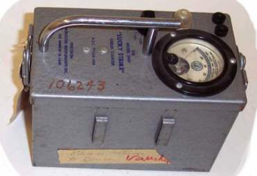
Let X equal the number of alpha particles emitted from barium-133 in 0.1 seconds and counted by a Geiger counter. One hundred observations of X produced these data.
It is claimed that X follows a Poisson distribution. Use a chi-square goodness-of-fit statistic to test whether this is true.
Answer
Note that very few observations resulted in 0, 1, or 2 alpha particles being emitted in 0.1 second. And, very few observations resulted in 10, 11, or 12 alpha particles being emitted in 0.1 second. Therefore, let's "collapse" the data at the two ends, yielding us nine "not-so-sparse" categories:
| Category | \(X\) | Obs'd |
|---|---|---|
| 1 | 0,1,2* | 5 |
| 2 | 3 | 13 |
| 3 | 4 | 19 |
| 4 | 5 | 16 |
| 5 | 6 | 15 |
| 6 | 7 | 9 |
| 7 | 8 | 12 |
| 8 | 9 | 7 |
| 9 | 10,11,12* | 4 |
| \(n = 100\) |
Because \(\lambda\), the mean of X, is not specified, we can estimate it with its maximum likelihood estimator, namely, the sample mean. Using the data, we get:
\(\bar{x}=\dfrac{1(1)+2(4)+3(13)+ ... + 12(1)}{100}=\dfrac{559}{100}=5.6\)
We can now estimate the probability that an observation will fall into each of the categories. The probability of falling into category 1, for example, is:
\(P(\{1\})=P(X=0)+P(X=1)+P(X=2) =\dfrac{e^{-5.6}5.6^0}{0!}+\dfrac{e^{-5.6}5.6^1}{1!}+\dfrac{e^{-5.6}5.6^2}{2!}=0.0824 \)
Here's what our table looks like now, after adding a column containing the estimated probabilities:
| Category | \(X\) | Obs'd | \(p_i = \left(e^{-5.6}5.6^x\right) / x!\) |
|---|---|---|---|
| 1 | 0,1,2* | 5 | 0.0824 |
| 2 | 3 | 13 | 0.1082 |
| 3 | 4 | 19 | 0.1515 |
| 4 | 5 | 16 | 0.1697 |
| 5 | 6 | 15 | 0.1584 |
| 6 | 7 | 9 | 0.1267 |
| 7 | 8 | 12 | 0.0887 |
| 8 | 9 | 7 | 0.0552 |
| 9 | 10,11,12* | 4 | 0.0539 |
| \(n = 100\) |
Now, we just have to add a column containing the expected number falling into each category. The expected number falling into category 1, for example, is 0.0824 × 100 = 8.24. Doing a similar calculation for each of the categories, we can add our column of expected numbers:
| Category | \(X\) | Obs'd | \(p_i = \left(e^{-5.6}5.6^x\right) / x!\) | Exp'd |
|---|---|---|---|---|
| 1 | 0,1,2* | 5 | 0.0824 | 8.24 |
| 2 | 3 | 13 | 0.1082 | 10.82 |
| 3 | 4 | 19 | 0.1515 | 15.15 |
| 4 | 5 | 16 | 0.1697 | 16.97 |
| 5 | 6 | 15 | 0.1584 | 15.84 |
| 6 | 7 | 9 | 0.1267 | 12.67 |
| 7 | 8 | 12 | 0.0887 | 8.87 |
| 8 | 9 | 7 | 0.0552 | 5.52 |
| 9 | 10,11,12* | 4 | 0.0539 | 5.39 |
| \(n = 100\) | 99.47 |
Now, we can use the observed numbers and the expected numbers to calculate our chi-square test statistic. Doing so, we get:
\(Q_{9-1}=\dfrac{(5-8.24)^2}{8.24}+\dfrac{(13-10.82)^2}{10.82}+ ... +\dfrac{(4-5.39)^2}{5.39}=5.7157 \)
Because we estimated d = 1 parameter, we need to compare our chi-square statistic to a chi-square distribution with (9−1)−1 = 7 degrees of freedom. That is, our critical region is defined as:
\(\text{Reject } H_0 \text{ if } Q_8 \ge \chi_{8-1, 0.05}^{2}=\chi_{7, 0.05}^{2}=14.07 \)
Because our test statistic doesn't fall in the rejection region, that is:
\(Q_8=5.77157 < \chi_{7, 0.05}^{2}=14.07\)
we fail to reject the null hypothesis. There is insufficient evidence at the 0.05 level to conclude that the data don't fit a Poisson probability model.