16.4 - Continuous Random Variables
16.4 - Continuous Random VariablesWhat if we are interested in using a chi-square goodness-of-fit test to see if our data follow some continuous distribution? That is, what if we want to test:
\( H_0 : F(w) =F_0(w)\)
where \(F_0 (w)\) is some known, specified distribution. Clearly, in this situation, it is no longer obvious what constitutes each of the categories. Perhaps we could all agree that the logical thing to do would be to divide up the interval of possible values into k "buckets" or "categories," called \(A_1, A_2, \dots, A_k\), say, into which the observed data can fall. Letting \(Y_i\) denote the number of times the observed value of W belongs to bucket \(A_i, i = 1, 2, \dots, k\), the random variables \(Y_1, Y_2, \dots, Y_k\) follow a multinomial distribution with parameters \(n, p_1, p_2, \dots, p_{k−1}\). The hypothesis that we actually test is a modification of the null hypothesis above, namely:
\(H_{0}^{'} : p_i = p_{i0}, i=1, 2, \dots , k \)
The hypothesis is rejected if the observed value of the chi-square statistic:
\(Q_{k-1} =\sum_{i=1}^{k}\frac{(Obs_i - Exp_i)^2}{Exp_i}\)
is at least as great as \(\chi_{\alpha}^{2}(k-1)\). If the hypothesis \(H_{0}^{'} : p_i = p_{i0}, i=1, 2, \dots , k\) is not rejected, then we do not reject the original hypothesis \(H_0 : F(w) =F_0(w)\) .
Let's make this proposed procedure more concrete by taking a look at an example.
Example 16-7
The IQs of one-hundred randomly selected people were determined using the Stanford-Binet Intelligence Quotient Test. The resulting data were, in sorted order, as follows:
| 54 | 66 | 74 | 74 | 75 | 78 | 79 | 80 | 81 | 82 |
|---|---|---|---|---|---|---|---|---|---|
| 82 | 82 | 83 | 84 | 87 | 88 | 88 | 88 | 88 | 89 |
| 89 | 89 | 89 | 89 | 90 | 90 | 90 | 91 | 92 | 93 |
| 93 | 93 | 94 | 96 | 96 | 97 | 97 | 98 | 98 | 99 |
| 99 | 99 | 99 | 99 | 100 | 100 | 100 | 102 | 102 | 102 |
| 102 | 102 | 103 | 103 | 104 | 104 | 104 | 105 | 105 | 105 |
| 105 | 106 | 106 | 106 | 107 | 107 | 108 | 108 | 108 | 109 |
| 109 | 109 | 110 | 111 | 111 | 111 | 111 | 112 | 112 | 112 |
| 114 | 114 | 115 | 115 | 115 | 116 | 118 | 118 | 120 | 121 |
| 121 | 122 | 123 | 125 | 126 | 127 | 127 | 131 | 132 | 139 |
Test the null hypothesis that the data come from a normal distribution with a mean of 100 and a standard deviation of 16.
Answer
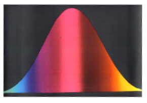
Hmm. So, where do we start? Well, we first have to define some categories. Let's divide up the interval of possible IQs into \(k = 10\) sets of equal probability \(\dfrac{1}{k} = \dfrac{1}{10}\). Perhaps this is best seen pictorially:
So, what's going on in this picture? Well, first the normal density is divided up into 10 intervals of equal probability (0.10). Well, okay, so the picture is not drawn very well to scale. At any rate, we then find the IQs that correspond to the \(k = 10\) cumulative probabilities of 0.1, 0.2, 0.3, etc. This is done in two steps:
- Step 1
first by finding the Z-scores associated with the cumulative probabilities 0.1, 0.2, 0.3, etc.
- Step 2
then by converting each Z-score into an X-value. It is those X-values (IQs) that will make up the "right-hand side" of each bucket:
Category \(X\) Obs'd \(p_i = \left(e^{-5.6}5.6^x\right) / x!\) Exp'd 1 0,1,2* 5 0.0824 8.24 2 3 13 0.1082 10.82 3 4 19 0.1515 15.15 4 5 16 0.1697 16.97 5 6 15 0.1584 15.84 6 7 9 0.1267 12.67 7 8 12 0.0887 8.87 8 9 7 0.0552 5.52 9 10,11,12* 4 0.0539 5.39 \(n = 100\) 99.47 -
Now, it's just a matter of counting the number of observations that fall into each bucket to get the observed (Obs'd) column, and calculating the expected number (0.10 × 100 = 10) to get the expected (Exp'd) column:Category Class 1 (\(-\infty\),79.5) 2 (79.5, 86.5) 3 (86.5, 91.6) 4 (91.6, 95.9) 5 (95.9, 100.0) 6 (100.0, 104.1) 7 (104.1, 108.4) 8 (108.4, 113.5) 9 (113.5, 120.5) 10 (120.5, \(\infty\))
-
| Category | Class | Obs'd | Exp'd | Contribution to \(Q\) |
|---|---|---|---|---|
| 1 | (\(-\infty\),79.5) | 7 | 10 | \(\left(7-10\right)^2 / 10 = 0.9\) |
| 2 | (79.5, 86.5) | 7 | 10 | \(\left(7-10\right)^2 / 10 = 0.9\) |
| 3 | (86.5, 91.6) | 14 | 10 | \(\left(14-10\right)^2 / 10 = 1.6\) |
| 4 | (91.6, 95.9) | 5 | 10 | \(\left(5-10\right)^2 / 10 = 2.5\) |
| 5 | (95.9, 100.0) | 14 | 10 | \(\left(14-10\right)^2 / 10 = 1.6\) |
| 6 | (100.0, 104.1) | 10 | 10 | \(\left(10-10\right)^2 / 10 = 0.0\) |
| 7 | (104.1, 108.4) | 12 | 10 | \(\left(12-10\right)^2 / 10 = 0.4\) |
| 8 | (108.4, 113.5) | 11 | 10 | \(\left(11-10\right)^2 / 10 = 0.1\) |
| 9 | (113.5, 120.5) | 9 | 10 | \(\left(9-10\right)^2 / 10 = 0.1\) |
| 10 | (120.5, \(\infty\)) | 11 | 10 | \(\left(11-10\right)^2 / 10 = 0.1\) |
| \(n = 100\) | \(n = 100\) | \(Q_9 = 8.2\) |
As illustrated in the table, using the observed and expected numbers, we see that the chi-square statistic is 8.2. We reject if the following is true:
\(Q_9 =8.2 \ge \chi_{10-1, 0.05}^{2} =\chi_{9, 0.05}^{2}=16.92\)
It isn't! We do not reject the null hypothesis at the 0.05 level. There is insufficient evidence to conclude that the data do not follow a normal distribution with a mean of 100 and a standard deviation 16.