7.6 - Using Minitab to Lighten the Workload
7.6 - Using Minitab to Lighten the WorkloadLeast Squares Regression Line
There are (at least) two ways that we can ask Minitab to calculate a least squares regression line for us. Let's use the height and weight example from the last page to illustrate. In either case, we first need to enter the data into two columns, as follows:
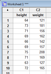
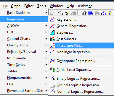
Now, the first method involves asking Minitab to create a fitted line plot. You can find the fitted line plot under the Stat menu. Select Stat >> Regression >> Fitted Line Plot..., as illustrated here:
In the pop-up window that appears, tell Minitab which variable is the Response (Y) and which variable is the Predictor (X). In our case, we select weight as the response, and height as the predictor:
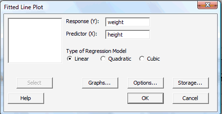
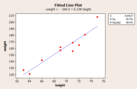
Then, select OK. A new graphics window should appear containing not only an equation, but also a graph, of the estimated regression line:
The second method involves asking Minitab to perform a regression analysis. You can find regression, again, under the Stat menu. Select Stat >>Regression >> Regression..., as illustrated here:
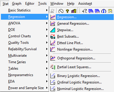
In the pop-up window that appears, again tell Minitab which variable is the Response (Y) and which variable is the Predictor (X). In our case, we again select weight as the response, and height as the predictor:
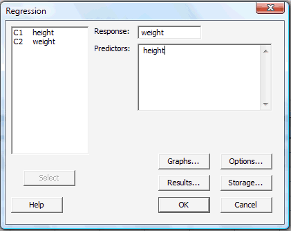
Then, select OK. The resulting analysis:
| The regression equation is weight = - 267 - 6.14 height |
||||
|---|---|---|---|---|
| Predictor | Coef | SE Coef | T | P |
| Constant | -266.53 | 51.03 | -5.22 | 0.001 |
| height | 6.1376 | 0.7353 | 8.35 | 0.000 |
|
|
|
|||
| S = 8.641 | R-Sq = 89.7% | R-Sq(adj) = 88.4% | ||
should appear in the Session window. You may have to page up in the Session window to see all of the analysis. (The above output just shows part of the analysis, with the portion pertaining to the estimated regression line highlighted in bold and blue.)
Now, as mentioned earlier, Minitab, by default, estimates the regression equation of the form:
\(\hat{y}_i=a_1+bx_i\)
It's easy enough to get Minitab to estimate the regression equation of the form:
\(\hat{y}_i=a+b(x_i-\bar{x})\)
We can first ask Minitab to calculate \(\bar{x}\) the mean height of the 10 students. The easiest way is to ask Minitab to calculate column statistics on the data in the height column. Select Calc >> Column Statistics...:
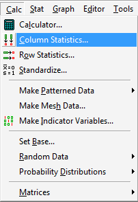
Then, select Mean, tell Minitab that the Input variable is height:
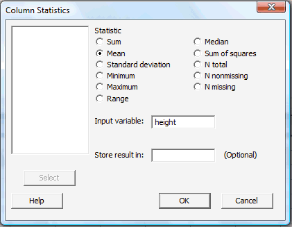
When you select OK, Minitab will display the results in the Session window:

Now, using the fact that the mean height is 69.3 inches, we need to calculate a new variable called, say, height* that equals height minus 69.3. We can do that using Minitab's calculator. First, label an empty column, C3, say height*:
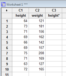
Then, under Calc, select Calculator...:

Use the calculator that appears in the pop-up window to tell Minitab to make the desired calculation:
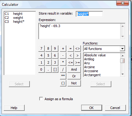
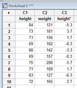
When you select OK, Minitab will enter the newly calculated data in the column labeled height*:
Now, it's just a matter of asking Minitab to performing another regression analysis... this time with the response as weight and the predictor as height*. Upon doing so, the resulting fitted line plot looks like this:
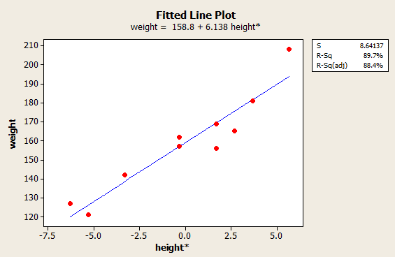
and the resulting regression analysis looks like this (with the portion pertaining to the estimated regression line highlighted in bold and blue):
| The regression equation is weight = 159 + 6.14 height* |
||||
|---|---|---|---|---|
| Predictor | Coef | SE Coef | T | P |
| Constant | 158.800 | 2.733 | 58.11 | 0.000 |
| height* | 6.1376 | 0.7353 | 8.35 | 0.000 |
|
|
|
|||
| S = 8.641 | R-Sq = 89.7% | R-Sq(adj) = 88.4% | ||
Estimating the Variance \(\sigma^2\)
You might not have noticed it, but we've already asked Minitab to estimate the common variance \(\sigma^2\)... or perhaps it's more accurate to say that Minitab calculates an estimate of the variance \(\sigma^2\), by default, every time it creates a fitted line plot or conducts a regression analysis. Here's where you'll find an estimate of the variance in the fitted line plot of our weight and height* data:
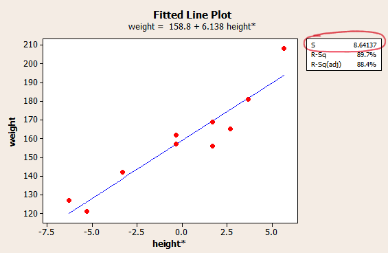
Well, okay, it would have been more accurate to say an estimate of the standard deviation \(\sigma\). We can simply square the estimate \(S\) (8.64137) to get the estimate \(S^2\) (74.67) of the variance \(\sigma^2\).
And, here's where you'll find an estimate of the variance in the fitted line plot of our weight and height data:
| The regression equation is weight = - 267 - 6.14 height |
||||
|---|---|---|---|---|
| Predictor | Coef | SE Coef | T | P |
| Constant | -266.53 | 51.03 | -5.22 | 0.001 |
| height | 6.1376 | 0.7353 | 8.35 | 0.000 |
|
|
|
|||
| S = 8.641 | R-Sq = 89.7% | R-Sq(adj) = 88.4% | ||
| Analysis of Variance | |||||
|---|---|---|---|---|---|
| Source | DF | SS | MS | F | P |
| Regression | 1 | 5202.2 | 5202.2 | 69.67 | 0.000 |
| Residual Error | 8 | 597.4 | 74.4 | 0.000 | |
|
Total |
9 | 5799.6 |
|
||
Here, we can see where Minitab displays not only \(S\), the estimate of the population standard deviation \(\sigma\), but also MSE (the Mean Square Error), the estimate of the population variance \(\sigma^2\). By the way, we shouldn't be surprised that the estimate of the variance is the same regardless of whether we use height or height* as the predictor. Right?