24.3 - Exponential Form
24.3 - Exponential FormYou might not have noticed that in all of the examples we have considered so far in this lesson, every p.d.f. or p.m.f. could we written in what is often called exponential form, that is:
\( f(x;\theta) =exp\left[K(x)p(\theta) + S(x) + q(\theta) \right] \)
with
- \(K(x)\) and \(S(x)\) being functions only of \(x\),
- \(p(\theta)\) and \(q(\theta)\) being functions only of the parameter \(\theta\)
- The support being free of the parameter \(\theta\).
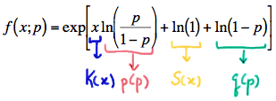
First, we had Bernoulli random variables with p.m.f. written in exponential form as:

with:
- \(K(x)\) and \(S(x)\) being functions only of \(x\),
- \(p(p)\) and \(q(p)\) being functions only of the parameter \(p\)
- The support \(x=0\), 1 not depending on the parameter \(p\)
Okay, we just skipped a lot of steps in that second equality sign, that is, in getting from point A (the typical p.m.f.) to point B (the p.m.f. written in exponential form). So, let's take a look at that more closely. We start with:
\( f(x;p) =p^x(1-p)^{1-x} \)
Is the p.m.f. in exponential form? Doesn't look like it to me! We clearly need an "exp" to appear up front. The only way we are going to get that without changing the underlying function is by taking the inverse function, that is, the natural log ("ln"), at the same time. Doing so, we get:
\( f(x;p) =exp\left[\text{ln}(p^x(1-p)^{1-x}) \right] \)
Is the p.m.f. now in exponential form? Nope, not yet, but at least it's looking more hopeful. All of the steps that follow now involve using what we know about the properties of logarithms. Recognizing that the natural log of a product is the sum of the natural logs, we get:
\( f(x;p) =exp\left[\text{ln}(p^x) + \text{ln}(1-p)^{1-x} \right] \)
Is the p.m.f. now in exponential form? Nope, still not yet, because \(K(x)\), \(p(p)\), \(S(x)\), and \(q(p)\) can't yet be identified as following exponential form, but we are certainly getting closer. Recognizing that the log of a power is the power times the log of the base, we get:
\( f(x;p) =exp\left[x\text{ln}(p) + (1-x)\text{ln}(1-p) \right] \)
This is getting tiring. Is the p.m.f. in exponential form yet? Nope, afraid not yet. Let's distribute that \((1-x)\) in that last term. Doing so, we get:
\( f(x;p) =exp\left[x\text{ln}(p) + \text{ln}(1-p) - x\text{ln}(1-p) \right] \)
Is the p.m.f. now in exponential form? Let's take a closer look. Well, in the first term, we can identify the \(K(x)p(p)\) and in the middle term, we see a function that depends only on the parameter \(p\):

Now, all we need is the last term to depend only on \(x\) and we're as good as gold. Oh, rats! The last term depends on both \(x\) and \(p\). So back to work some more! Recognizing that the log of a quotient is the difference between the logs of the numerator and denominator, we get:
\( f(x;p) =exp\left[x\text{ln}\left( \frac{p}{1-p}\right) + \text{ln}(1-p) \right] \)
Is the p.m.f. now in exponential form? So close! Let's just add 0 in (by way of the natural log of 1) to make it obvious. Doing so, we get:
\( f(x;p) =exp\left[x\text{ln}\left( \frac{p}{1-p}\right) + \text{ln}(1) + \text{ln}(1-p) \right] \)
Yes, we have finally written the Bernoulli p.m.f. in exponential form:

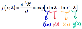
Whew! So, we've fully explored writing the Bernoulli p.m.f. in exponential form! Let's get back to reviewing all of the p.m.f.'s we've encountered in this lesson. We had Poisson random variables whose p.m.f. can be written in exponential form as:

with
- \(K(x)\) and \(S(x)\) being functions only of \(x\),
- \(p(\lambda)\) and \(q(\lambda)\) being functions only of the parameter \(\lambda\)
- The support \(x = 0, 1, 2, \ldots\) not depending on the parameter \(\lambda\)
Then, we had \(N(\mu, 1)\) random variables whose p.d.f. can be written in exponential form as:

with
- \(K(x)\) and \(S(x)\) being functions only of \(x\),
- \(p(\mu)\) and \(q(\mu)\) being functions only of the parameter \(\mu\)
- The support \(-\infty<x<\infty\) not depending on the parameter \(\mu\)
Then, we had exponential random variables random variables whose p.d.f. can be written in exponential form as:

with
- \(K(x)\) and \(S(x)\) being functions only of \(x\),
- \(p(\theta)\) and \(q(\theta)\) being functions only of the parameter \(\theta\)
- The support \(x\ge 0\) not depending on the parameter \(\theta\).
Happily, it turns out that writing p.d.f.s and p.m.f.s in exponential form provides us yet a third way of identifying sufficient statistics for our parameters. The following theorem tells us how.
Exponential Criterion:
Let \(X_1, X_2, \ldots, X_n\) be a random sample from a distribution with a p.d.f. or p.m.f. of the exponential form:
\( f(x;\theta) =exp\left[K(x)p(\theta) + S(x) + q(\theta) \right] \)
with a support that does not depend on \(\theta\). Then, the statistic:
\( \sum_{i=1}^{n} K(X_i) \)
is sufficient for \(\theta\).
Proof
Because \(X_1, X_2, \ldots, X_n\) is a random sample, the joint p.d.f. (or joint p.m.f.) of \(X_1, X_2, \ldots, X_n\) is, by independence:
\(f(x_1, x_2, ... , x_n;\theta)= f(x_1;\theta) \times f(x_2;\theta) \times ... \times f(x_n;\theta) \)
Inserting what we know to be the p.m.f. or p.d.f. in exponential form, we get:
\(f(x_1, ... , x_n;\theta)=\text{exp}\left[K(x_1)p(\theta) + S(x_1)+q(\theta)\right] \times ... \times \text{exp}\left[K(x_n)p(\theta) + S(x_n)+q(\theta)\right] \)
Collecting like terms in the exponents, we get:
\(f(x_1, ... , x_n;\theta)=\text{exp}\left[p(\theta)\sum_{i=1}^{n}K(x_i) + \sum_{i=1}^{n}S(x_i) + nq(\theta)\right] \)
which can be factored as:
\(f(x_1, ... , x_n;\theta)=\left\{ \text{exp}\left[p(\theta)\sum_{i=1}^{n}K(x_i) + nq(\theta)\right]\right\} \times \left\{ \text{exp}\left[\sum_{i=1}^{n}S(x_i)\right] \right\} \)
We have factored the joint p.m.f. or p.d.f. into two functions, one (\(\phi\)) being only a function of the statistic \(Y=\sum_{i=1}^{n}K(X_i)\) and the other (h) not depending on the parameter \(\theta\):

Therefore, the Factorization Theorem tells us that \(Y=\sum_{i=1}^{n}K(X_i)\) is a sufficient statistic for \(\theta\).
Let's try the Exponential Criterion out on an example.
Example 24-5

Let \(X_1, X_2, \ldots, X_n\) be a random sample from a geometric distribution with parameter \(p\). Find a sufficient statistic for the parameter \(p\).
Answer
The probability mass function of a geometric random variable is:
\(f(x;p) = (1-p)^{x-1}p\)
for \(x=1, 2, 3, \ldots\) The p.m.f. can be written in exponential form as:
\(f(x;p) = \text{exp}\left[ x\text{log}(1-p)+\text{log}(1)+\text{log}\left( \frac{p}{1-p} \right)\right] \)
Therefore, \(Y=\sum_{i=1}^{n}X_i\) is sufficient for \(p\). Easy as pie!
By the way, you might want to note that almost every p.m.f. or p.d.f. we encounter in this course can be written in exponential form. With that noted, you might want to make the Exponential Criterion the first tool you grab out of your toolbox when trying to find a sufficient statistic for a parameter.