Lesson 1: Point Estimation

Overview

Suppose we have an unknown population parameter, such as a population mean $\mu$ or a population proportion $p$, which we'd like to estimate. For example, suppose we are interested in estimating:

$p$ = the (unknown) proportion of American college students, 18-24, who have a smart phone
$\mu$ = the (unknown) mean number of days it takes Alzheimer's patients to achieve certain milestones

In either case, we can't possibly survey the entire population. That is, we can't survey all American college students between the ages of 18 and 24. Nor can we survey all patients with Alzheimer's disease. So, of course, we do what comes naturally and take a random sample from the population, and use the resulting data to estimate the value of the population parameter. Of course, we want the estimate to be "good" in some way.

In this lesson, we'll learn two methods, namely the method of maximum likelihood and the method of moments, for deriving formulas for "good" point estimates for population parameters. We'll also learn one way of assessing whether a point estimate is "good." We'll do that by defining what a means for an estimate to be unbiased.

Objectives

Upon completion of this lesson, you should be able to:

To learn how to find a maximum likelihood estimator of a population parameter.
To learn how to find a method of moments estimator of a population parameter.
To learn how to check to see if an estimator is unbiased for a particular parameter.
To understand the steps involved in each of the proofs in the lesson.
To be able to apply the methods learned in the lesson to new problems.

1.1 - Definitions

We'll start the lesson with some formal definitions. In doing so, recall that we denote the $n$ random variables arising from a random sample as subscripted uppercase letters:

$X_1, X_2, \cdots, X_n$

The corresponding observed values of a specific random sample are then denoted as subscripted lowercase letters:

$x_1, x_2, \cdots, x_n$

Parameter Space: The range of possible values of the parameter $\theta$ is called the parameter space $\Omega$ (the greek letter "omega").

For example, if $\mu$ denotes the mean grade point average of all college students, then the parameter space (assuming a 4-point grading scale) is:

$\Omega=\{\mu: 0\le \mu\le 4\}$

And, if $p$ denotes the proportion of students who smoke cigarettes, then the parameter space is:

$\Omega=\{p:0\le p\le 1\}$

Point Estimator: The function of $X_1, X_2, \cdots, X_n$, that is, the statistic $u=(X_1, X_2, \cdots, X_n)$, used to estimate $\theta$ is called a point estimator of $\theta$.

For example, the function:

$\bar{X}=\dfrac{1}{n}\sum\limits_{i=1}^n X_i$

is a point estimator of the population mean $\mu$. The function:

$\hat{p}=\dfrac{1}{n}\sum\limits_{i=1}^n X_i$

(where $X_i=0\text{ or }1)$ is a point estimator of the population proportion $p$. And, the function:

$S^2=\dfrac{1}{n-1}\sum\limits_{i=1}^n (X_i-\bar{X})^2$

is a point estimator of the population variance $\sigma^2$.

Point Estimate: The function $u(x_1, x_2, \cdots, x_n)$ computed from a set of data is an observed point estimate of $\theta$.

For example, if $x_i$ are the observed grade point averages of a sample of 88 students, then:

$\bar{x}=\dfrac{1}{88}\sum\limits_{i=1}^{88} x_i=3.12$

is a point estimate of $\mu$, the mean grade point average of all the students in the population.

And, if $x_i=0$ if a student has no tattoo, and $x_i=1$ if a student has a tattoo, then:

$\hat{p}=0.11$

is a point estimate of $p$, the proportion of all students in the population who have a tattoo.

Now, with the above definitions aside, let's go learn about the method of maximum likelihood.

1.2 - Maximum Likelihood Estimation

Statement of the Problem

Suppose we have a random sample $X_1, X_2, \cdots, X_n$ whose assumed probability distribution depends on some unknown parameter $\theta$. Our primary goal here will be to find a point estimator $u(X_1, X_2, \cdots, X_n)$, such that $u(x_1, x_2, \cdots, x_n)$ is a "good" point estimate of $\theta$, where $x_1, x_2, \cdots, x_n$ are the observed values of the random sample. For example, if we plan to take a random sample $X_1, X_2, \cdots, X_n$ for which the $X_i$ are assumed to be normally distributed with mean $\mu$ and variance $\sigma^2$, then our goal will be to find a good estimate of $\mu$, say, using the data $x_1, x_2, \cdots, x_n$ that we obtained from our specific random sample.

The Basic Idea

It seems reasonable that a good estimate of the unknown parameter $\theta$ would be the value of $\theta$ that maximizes the probability, errrr... that is, the likelihood... of getting the data we observed. (So, do you see from where the name "maximum likelihood" comes?) So, that is, in a nutshell, the idea behind the method of maximum likelihood estimation. But how would we implement the method in practice? Well, suppose we have a random sample $X_1, X_2, \cdots, X_n$ for which the probability density (or mass) function of each $X_i$ is $f(x_i;\theta)$. Then, the joint probability mass (or density) function of $X_1, X_2, \cdots, X_n$, which we'll (not so arbitrarily) call $L(\theta)$ is:

$L(\theta)=P(X_1=x_1,X_2=x_2,\ldots,X_n=x_n)=f(x_1;\theta)\cdot f(x_2;\theta)\cdots f(x_n;\theta)=\prod\limits_{i=1}^n f(x_i;\theta)$

The first equality is of course just the definition of the joint probability mass function. The second equality comes from that fact that we have a random sample, which implies by definition that the $X_i$ are independent. And, the last equality just uses the shorthand mathematical notation of a product of indexed terms. Now, in light of the basic idea of maximum likelihood estimation, one reasonable way to proceed is to treat the "likelihood function" $L(\theta)$ as a function of $\theta$, and find the value of $\theta$ that maximizes it.

Is this still sounding like too much abstract gibberish? Let's take a look at an example to see if we can make it a bit more concrete.

Example 1-1

Suppose we have a random sample $X_1, X_2, \cdots, X_n$ where:

$X_i=0$ if a randomly selected student does not own a sports car, and
$X_i=1$ if a randomly selected student does own a sports car.

Assuming that the $X_i$ are independent Bernoulli random variables with unknown parameter $p$, find the maximum likelihood estimator of $p$, the proportion of students who own a sports car.

Answer

If the $X_i$ are independent Bernoulli random variables with unknown parameter $p$, then the probability mass function of each $X_i$ is:

$f(x_i;p)=p^{x_i}(1-p)^{1-x_i}$

for $x_i=0$ or 1 and $0<p<1$. Therefore, the likelihood function $L(p)$ is, by definition:

$L(p)=\prod\limits_{i=1}^n f(x_i;p)=p^{x_1}(1-p)^{1-x_1}\times p^{x_2}(1-p)^{1-x_2}\times \cdots \times p^{x_n}(1-p)^{1-x_n}$

for $0<p<1$. Simplifying, by summing up the exponents, we get :

$L(p)=p^{\sum x_i}(1-p)^{n-\sum x_i}$

Now, in order to implement the method of maximum likelihood, we need to find the $p$ that maximizes the likelihood $L(p)$. We need to put on our calculus hats now since, in order to maximize the function, we are going to need to differentiate the likelihood function with respect to $p$. In doing so, we'll use a "trick" that often makes the differentiation a bit easier. Note that the natural logarithm is an increasing function of $x$:

That is, if $x_1<x_2$, then $f(x_1)<f(x_2)$. That means that the value of $p$ that maximizes the natural logarithm of the likelihood function $\ln L(p)$ is also the value of $p$ that maximizes the likelihood function $L(p)$. So, the "trick" is to take the derivative of $\ln L(p)$ (with respect to $p$) rather than taking the derivative of $L(p)$. Again, doing so often makes the differentiation much easier. (By the way, throughout the remainder of this course, I will use either $\ln L(p)$ or $\log L(p)$ to denote the natural logarithm of the likelihood function.)

In this case, the natural logarithm of the likelihood function is:

$\text{log}L(p)=(\sum x_i)\text{log}(p)+(n-\sum x_i)\text{log}(1-p)$

Now, taking the derivative of the log-likelihood, and setting it to 0, we get:

$\displaystyle{\frac{\partial \log L(p)}{\partial p}=\frac{\sum x_{i}}{p}-\frac{\left(n-\sum x_{i}\right)}{1-p} \stackrel{SET}{\equiv} 0}$

Now, multiplying through by $p(1-p)$, we get:

$(\sum x_i)(1-p)-(n-\sum x_i)p=0$

Upon distribution, we see that two of the resulting terms cancel each other out:

$\sum x_{i} - \color{red}\cancel {\color{black}p \sum x_{i}} \color{black}-n p+ \color{red}\cancel {\color{black} p \sum x_{i}} \color{black} = 0$

leaving us with:

$\sum x_i-np=0$

Now, all we have to do is solve for $p$. In doing so, you'll want to make sure that you always put a hat ("^") on the parameter, in this case, $p$, to indicate it is an estimate:

$\hat{p}=\dfrac{\sum\limits_{i=1}^n x_i}{n}$

or, alternatively, an estimator:

$\hat{p}=\dfrac{\sum\limits_{i=1}^n X_i}{n}$

Oh, and we should technically verify that we indeed did obtain a maximum. We can do that by verifying that the second derivative of the log-likelihood with respect to $p$ is negative. It is, but you might want to do the work to convince yourself!

Now, with that example behind us, let us take a look at formal definitions of the terms:

Likelihood function
Maximum likelihood estimators
Maximum likelihood estimates.

Definition. Let $X_1, X_2, \cdots, X_n$ be a random sample from a distribution that depends on one or more unknown parameters $\theta_1, \theta_2, \cdots, \theta_m$with probability density (or mass) function $f(x_i; \theta_1, \theta_2, \cdots, \theta_m)$. Suppose that $(\theta_1, \theta_2, \cdots, \theta_m)$ is restricted to a given parameter space $\Omega$. Then:

When regarded as a function of $\theta_1, \theta_2, \cdots, \theta_m$, the joint probability density (or mass) function of $X_1, X_2, \cdots, X_n$:

$L(\theta_1,\theta_2,\ldots,\theta_m)=\prod\limits_{i=1}^n f(x_i;\theta_1,\theta_2,\ldots,\theta_m)$

($(\theta_1, \theta_2, \cdots, \theta_m)$ in $\Omega$) is called the likelihood function.
If:

$[u_1(x_1,x_2,\ldots,x_n),u_2(x_1,x_2,\ldots,x_n),\ldots,u_m(x_1,x_2,\ldots,x_n)]$

is the $m$-tuple that maximizes the likelihood function, then:

$\hat{\theta}_i=u_i(X_1,X_2,\ldots,X_n)$

is the maximum likelihood estimator of $\theta_i$, for $i=1, 2, \cdots, m$.
The corresponding observed values of the statistics in (2), namely:

$[u_1(x_1,x_2,\ldots,x_n),u_2(x_1,x_2,\ldots,x_n),\ldots,u_m(x_1,x_2,\ldots,x_n)]$

are called the maximum likelihood estimates of $\theta_i$, for $i=1, 2, \cdots, m$.

Example 1-2

Suppose the weights of randomly selected American female college students are normally distributed with unknown mean $\mu$ and standard deviation $\sigma$. A random sample of 10 American female college students yielded the following weights (in pounds):

115 122 130 127 149 160 152 138 149 180

Based on the definitions given above, identify the likelihood function and the maximum likelihood estimator of $\mu$, the mean weight of all American female college students. Using the given sample, find a maximum likelihood estimate of $\mu$ as well.

Answer

The probability density function of $X_i$ is:

$f(x_i;\mu,\sigma^2)=\dfrac{1}{\sigma \sqrt{2\pi}}\text{exp}\left[-\dfrac{(x_i-\mu)^2}{2\sigma^2}\right]$

for $-\infty<x<\infty$. The parameter space is $\Omega=\{(\mu, \sigma):-\infty<\mu<\infty \text{ and }0<\sigma<\infty\}$. Therefore, (you might want to convince yourself that) the likelihood function is:

$L(\mu,\sigma)=\sigma^{-n}(2\pi)^{-n/2}\text{exp}\left[-\dfrac{1}{2\sigma^2}\sum\limits_{i=1}^n(x_i-\mu)^2\right]$

for $-\infty<\mu<\infty \text{ and }0<\sigma<\infty$. It can be shown (we'll do so in the next example!), upon maximizing the likelihood function with respect to $\mu$, that the maximum likelihood estimator of $\mu$ is:

$\hat{\mu}=\dfrac{1}{n}\sum\limits_{i=1}^n X_i=\bar{X}$

Based on the given sample, a maximum likelihood estimate of $\mu$ is:

$\hat{\mu}=\dfrac{1}{n}\sum\limits_{i=1}^n x_i=\dfrac{1}{10}(115+\cdots+180)=142.2$

pounds. Note that the only difference between the formulas for the maximum likelihood estimator and the maximum likelihood estimate is that:

the estimator is defined using capital letters (to denote that its value is random), and
the estimate is defined using lowercase letters (to denote that its value is fixed and based on an obtained sample)

Okay, so now we have the formal definitions out of the way. The first example on this page involved a joint probability mass function that depends on only one parameter, namely $p$, the proportion of successes. Now, let's take a look at an example that involves a joint probability density function that depends on two parameters.

Example 1-3

Let $X_1, X_2, \cdots, X_n$ be a random sample from a normal distribution with unknown mean $\mu$ and variance $\sigma^2$. Find maximum likelihood estimators of mean $\mu$ and variance $\sigma^2$.

Answer

In finding the estimators, the first thing we'll do is write the probability density function as a function of $\theta_1=\mu$ and $\theta_2=\sigma^2$:

$f(x_i;\theta_1,\theta_2)=\dfrac{1}{\sqrt{\theta_2}\sqrt{2\pi}}\text{exp}\left[-\dfrac{(x_i-\theta_1)^2}{2\theta_2}\right]$

for $-\infty<\theta_1<\infty \text{ and }0<\theta_2<\infty$. We do this so as not to cause confusion when taking the derivative of the likelihood with respect to $\sigma^2$. Now, that makes the likelihood function:

$ L(\theta_1,\theta_2)=\prod\limits_{i=1}^n f(x_i;\theta_1,\theta_2)=\theta^{-n/2}_2(2\pi)^{-n/2}\text{exp}\left[-\dfrac{1}{2\theta_2}\sum\limits_{i=1}^n(x_i-\theta_1)^2\right]$

and therefore the log of the likelihood function:

$\text{log} L(\theta_1,\theta_2)=-\dfrac{n}{2}\text{log}\theta_2-\dfrac{n}{2}\text{log}(2\pi)-\dfrac{\sum(x_i-\theta_1)^2}{2\theta_2}$

Now, upon taking the partial derivative of the log likelihood with respect to $\theta_1$, and setting to 0, we see that a few things cancel each other out, leaving us with:

$\displaystyle{\frac{\partial \log L\left(\theta_{1}, \theta_{2}\right)}{\partial \theta_{1}}=\frac{-\color{red} \cancel {\color{black}2} \color{black}\sum\left(x_{i}-\theta_{1}\right)\color{red}\cancel{\color{black}(-1)}}{\color{red}\cancel{\color{black}2} \color{black} \theta_{2}} \stackrel{\text { SET }}{\equiv} 0}$

Now, multiplying through by $\theta_2$, and distributing the summation, we get:

$\sum x_i-n\theta_1=0$

Now, solving for $\theta_1$, and putting on its hat, we have shown that the maximum likelihood estimate of $\theta_1$is:

$\hat{\theta}_1=\hat{\mu}=\dfrac{\sum x_i}{n}=\bar{x}$

Now for $\theta_2$. Taking the partial derivative of the log likelihood with respect to $\theta_2$, and setting to 0, we get:

$\displaystyle{\frac{\partial \log L\left(\theta_{1}, \theta_{2}\right)}{\partial \theta_{2}}=-\frac{n}{2 \theta_{2}}+\frac{\sum\left(x_{i}-\theta_{1}\right)^{2}}{2 \theta_{2}^{2}} \stackrel{\text { SET }}{\equiv} 0}$

Multiplying through by $2\theta^2_2$:

$\displaystyle{\frac{\partial \log L\left(\theta_{1}, \theta_{2}\right)}{\partial \theta_{1}}=\left[-\frac{n}{2 \theta_{2}}+\frac{\sum\left(x_{i}-\theta_{1}\right)^{2}}{2 \theta_{2}^{2}} \stackrel{s \epsilon \epsilon}{\equiv} 0\right] \times 2 \theta_{2}^{2}}$

we get:

$-n\theta_2+\sum(x_i-\theta_1)^2=0$

And, solving for $\theta_2$, and putting on its hat, we have shown that the maximum likelihood estimate of $\theta_2$is:

$\hat{\theta}_2=\hat{\sigma}^2=\dfrac{\sum(x_i-\bar{x})^2}{n}$

(I'll again leave it to you to verify, in each case, that the second partial derivative of the log likelihood is negative, and therefore that we did indeed find maxima.) In summary, we have shown that the maximum likelihood estimators of $\mu$ and variance $\sigma^2$ for the normal model are:

$\hat{\mu}=\dfrac{\sum X_i}{n}=\bar{X}$ and $\hat{\sigma}^2=\dfrac{\sum(X_i-\bar{X})^2}{n}$

respectively.

Note that the maximum likelihood estimator of $\sigma^2$ for the normal model is not the sample variance $S^2$. They are, in fact, competing estimators. So how do we know which estimator we should use for $\sigma^2$ ? Well, one way is to choose the estimator that is "unbiased." Let's go learn about unbiased estimators now.

1.3 - Unbiased Estimation

On the previous page, we showed that if $X_i$ are Bernoulli random variables with parameter $p$, then:

$\hat{p}=\dfrac{1}{n}\sum\limits_{i=1}^n X_i$

is the maximum likelihood estimator of $p$. And, if $X_i$ are normally distributed random variables with mean $\mu$ and variance $\sigma^2$, then:

$\hat{\mu}=\dfrac{\sum X_i}{n}=\bar{X}$ and $\hat{\sigma}^2=\dfrac{\sum(X_i-\bar{X})^2}{n}$

are the maximum likelihood estimators of $\mu$ and $\sigma^2$, respectively. A natural question then is whether or not these estimators are "good" in any sense. One measure of "good" is "unbiasedness."

Bias and Unbias Estimator

If the following holds:

$E[u(X_1,X_2,\ldots,X_n)]=\theta$

then the statistic $u(X_1,X_2,\ldots,X_n)$ is an unbiased estimator of the parameter $\theta$. Otherwise, $u(X_1,X_2,\ldots,X_n)$ is a biased estimator of $\theta$.

Example 1-4

If $X_i$ is a Bernoulli random variable with parameter $p$, then:

$\hat{p}=\dfrac{1}{n}\sum\limits_{i=1}^nX_i$

is the maximum likelihood estimator (MLE) of $p$. Is the MLE of $p$ an unbiased estimator of $p$?

Answer

Recall that if $X_i$ is a Bernoulli random variable with parameter $p$, then $E(X_i)=p$. Therefore:

$E(\hat{p})=E\left(\dfrac{1}{n}\sum\limits_{i=1}^nX_i\right)=\dfrac{1}{n}\sum\limits_{i=1}^nE(X_i)=\dfrac{1}{n}\sum\limits_{i=1}^np=\dfrac{1}{n}(np)=p$

The first equality holds because we've merely replaced $\hat{p}$ with its definition. The second equality holds by the rules of expectation for a linear combination. The third equality holds because $E(X_i)=p$. The fourth equality holds because when you add the value $p$ up $n$ times, you get $np$. And, of course, the last equality is simple algebra.

In summary, we have shown that:

$E(\hat{p})=p$

Therefore, the maximum likelihood estimator is an unbiased estimator of $p$.

Example 1-5

If $X_i$ are normally distributed random variables with mean $\mu$ and variance $\sigma^2$, then:

$\hat{\mu}=\dfrac{\sum X_i}{n}=\bar{X}$ and $\hat{\sigma}^2=\dfrac{\sum(X_i-\bar{X})^2}{n}$

are the maximum likelihood estimators of $\mu$ and $\sigma^2$, respectively. Are the MLEs unbiased for their respective parameters?

Answer

Recall that if $X_i$ is a normally distributed random variable with mean $\mu$ and variance $\sigma^2$, then $E(X_i)=\mu$ and $\text{Var}(X_i)=\sigma^2$. Therefore:

$E(\bar{X})=E\left(\dfrac{1}{n}\sum\limits_{i=1}^nX_i\right)=\dfrac{1}{n}\sum\limits_{i=1}^nE(X_i)=\dfrac{1}{n}\sum\limits_{i=1}\mu=\dfrac{1}{n}(n\mu)=\mu$

The first equality holds because we've merely replaced $\bar{X}$ with its definition. Again, the second equality holds by the rules of expectation for a linear combination. The third equality holds because $E(X_i)=\mu$. The fourth equality holds because when you add the value $\mu$ up $n$ times, you get $n\mu$. And, of course, the last equality is simple algebra.

In summary, we have shown that:

$E(\bar{X})=\mu$

Therefore, the maximum likelihood estimator of $\mu$ is unbiased. Now, let's check the maximum likelihood estimator of $\sigma^2$. First, note that we can rewrite the formula for the MLE as:

$\hat{\sigma}^2=\left(\dfrac{1}{n}\sum\limits_{i=1}^nX_i^2\right)-\bar{X}^2$

because:

$\displaystyle{\begin{aligned}
\hat{\sigma}^{2}=\frac{1}{n} \sum_{i=1}^{n}\left(x_{i}-\bar{x}\right)^{2} &=\frac{1}{n} \sum_{i=1}^{n}\left(x_{i}^{2}-2 x_{i} \bar{x}+\bar{x}^{2}\right) \\
&=\frac{1}{n} \sum_{i=1}^{n} x_{i}^{2}-2 \bar{x} \cdot \color{blue}\underbrace{\color{black}\frac{1}{n} \sum x_{i}}_{\bar{x}} \color{black} + \frac{1}{\color{blue}\cancel{\color{black} n}}\left(\color{blue}\cancel{\color{black}n} \color{black}\bar{x}^{2}\right) \\
&=\frac{1}{n} \sum_{i=1}^{n} x_{i}^{2}-\bar{x}^{2}
\end{aligned}}$

Then, taking the expectation of the MLE, we get:

$E(\hat{\sigma}^2)=\dfrac{(n-1)\sigma^2}{n}$

as illustrated here:

\begin{align} E(\hat{\sigma}^2) &= E\left[\dfrac{1}{n}\sum\limits_{i=1}^nX_i^2-\bar{X}^2\right]=\left[\dfrac{1}{n}\sum\limits_{i=1}^nE(X_i^2)\right]-E(\bar{X}^2)\\ &= \dfrac{1}{n}\sum\limits_{i=1}^n(\sigma^2+\mu^2)-\left(\dfrac{\sigma^2}{n}+\mu^2\right)\\ &= \dfrac{1}{n}(n\sigma^2+n\mu^2)-\dfrac{\sigma^2}{n}-\mu^2\\ &= \sigma^2-\dfrac{\sigma^2}{n}=\dfrac{n\sigma^2-\sigma^2}{n}=\dfrac{(n-1)\sigma^2}{n}\\ \end{align}

The first equality holds from the rewritten form of the MLE. The second equality holds from the properties of expectation. The third equality holds from manipulating the alternative formulas for the variance, namely:

$Var(X)=\sigma^2=E(X^2)-\mu^2$ and $Var(\bar{X})=\dfrac{\sigma^2}{n}=E(\bar{X}^2)-\mu^2$

The remaining equalities hold from simple algebraic manipulation. Now, because we have shown:

$E(\hat{\sigma}^2) \neq \sigma^2$

the maximum likelihood estimator of $\sigma^2$ is a biased estimator.

Example 1-6

If $X_i$ are normally distributed random variables with mean $\mu$ and variance $\sigma^2$, what is an unbiased estimator of $\sigma^2$? Is $S^2$ unbiased?

Answer

Recall that if $X_i$ is a normally distributed random variable with mean $\mu$ and variance $\sigma^2$, then:

$\dfrac{(n-1)S^2}{\sigma^2}\sim \chi^2_{n-1}$

Also, recall that the expected value of a chi-square random variable is its degrees of freedom. That is, if:

$X \sim \chi^2_{(r)}$

then $E(X)=r$. Therefore:

$E(S^2)=E\left[\dfrac{\sigma^2}{n-1}\cdot \dfrac{(n-1)S^2}{\sigma^2}\right]=\dfrac{\sigma^2}{n-1} E\left[\dfrac{(n-1)S^2}{\sigma^2}\right]=\dfrac{\sigma^2}{n-1}\cdot (n-1)=\sigma^2$

The first equality holds because we effectively multiplied the sample variance by 1. The second equality holds by the law of expectation that tells us we can pull a constant through the expectation. The third equality holds because of the two facts we recalled above. That is:

$E\left[\dfrac{(n-1)S^2}{\sigma^2}\right]=n-1$

And, the last equality is again simple algebra.

In summary, we have shown that, if $X_i$ is a normally distributed random variable with mean $\mu$ and variance $\sigma^2$, then $S^2$ is an unbiased estimator of $\sigma^2$. It turns out, however, that $S^2$ is always an unbiased estimator of $\sigma^2$, that is, for any model, not just the normal model. (You'll be asked to show this in the homework.) And, although $S^2$ is always an unbiased estimator of $\sigma^2$, $S$ is not an unbiased estimator of $\sigma$. (You'll be asked to show this in the homework, too.)

Sometimes it is impossible to find maximum likelihood estimators in a convenient closed form. Instead, numerical methods must be used to maximize the likelihood function. In such cases, we might consider using an alternative method of finding estimators, such as the "method of moments." Let's go take a look at that method now.

1.4 - Method of Moments

In short, the method of moments involves equating sample moments with theoretical moments. So, let's start by making sure we recall the definitions of theoretical moments, as well as learn the definitions of sample moments.

Definitions.

$E(X^k)$ is the $k^{th}$ (theoretical) moment of the distribution (about the origin), for $k=1, 2, \ldots$
$E\left[(X-\mu)^k\right]$ is the $k^{th}$ (theoretical) moment of the distribution (about the mean), for $k=1, 2, \ldots$
$M_k=\dfrac{1}{n}\sum\limits_{i=1}^n X_i^k$ is the $k^{th}$ sample moment, for $k=1, 2, \ldots$
$M_k^\ast =\dfrac{1}{n}\sum\limits_{i=1}^n (X_i-\bar{X})^k$ is the $k^{th}$ sample moment about the mean, for $k=1, 2, \ldots$

One Form of the Method

The basic idea behind this form of the method is to:

Equate the first sample moment about the origin $M_1=\dfrac{1}{n}\sum\limits_{i=1}^n X_i=\bar{X}$ to the first theoretical moment $E(X)$.
Equate the second sample moment about the origin $M_2=\dfrac{1}{n}\sum\limits_{i=1}^n X_i^2$ to the second theoretical moment $E(X^2)$.
Continue equating sample moments about the origin, $M_k$, with the corresponding theoretical moments $E(X^k), \; k=3, 4, \ldots$ until you have as many equations as you have parameters.
Solve for the parameters.

The resulting values are called method of moments estimators. It seems reasonable that this method would provide good estimates, since the empirical distribution converges in some sense to the probability distribution. Therefore, the corresponding moments should be about equal.

Example 1-7

Let $X_1, X_2, \ldots, X_n$ be Bernoulli random variables with parameter $p$. What is the method of moments estimator of $p$?

Answer

Here, the first theoretical moment about the origin is:

$E(X_i)=p$

We have just one parameter for which we are trying to derive the method of moments estimator. Therefore, we need just one equation. Equating the first theoretical moment about the origin with the corresponding sample moment, we get:

$p=\dfrac{1}{n}\sum\limits_{i=1}^n X_i$

Now, we just have to solve for $p$. Whoops! In this case, the equation is already solved for $p$. Our work is done! We just need to put a hat (^) on the parameter to make it clear that it is an estimator. We can also subscript the estimator with an "MM" to indicate that the estimator is the method of moments estimator:

$\hat{p}_{MM}=\dfrac{1}{n}\sum\limits_{i=1}^n X_i$

So, in this case, the method of moments estimator is the same as the maximum likelihood estimator, namely, the sample proportion.

Example 1-8

Let $X_1, X_2, \ldots, X_n$ be normal random variables with mean $\mu$ and variance $\sigma^2$. What are the method of moments estimators of the mean $\mu$ and variance $\sigma^2$?

Answer

The first and second theoretical moments about the origin are:

$E(X_i)=\mu\qquad E(X_i^2)=\sigma^2+\mu^2$

(Incidentally, in case it's not obvious, that second moment can be derived from manipulating the shortcut formula for the variance.) In this case, we have two parameters for which we are trying to derive method of moments estimators. Therefore, we need two equations here. Equating the first theoretical moment about the origin with the corresponding sample moment, we get:

$E(X)=\mu=\dfrac{1}{n}\sum\limits_{i=1}^n X_i$

And, equating the second theoretical moment about the origin with the corresponding sample moment, we get:

$E(X^2)=\sigma^2+\mu^2=\dfrac{1}{n}\sum\limits_{i=1}^n X_i^2$

Now, the first equation tells us that the method of moments estimator for the mean $\mu$ is the sample mean:

$\hat{\mu}_{MM}=\dfrac{1}{n}\sum\limits_{i=1}^n X_i=\bar{X}$

And, substituting the sample mean in for $\mu$ in the second equation and solving for $\sigma^2$, we get that the method of moments estimator for the variance $\sigma^2$ is:

$\hat{\sigma}^2_{MM}=\dfrac{1}{n}\sum\limits_{i=1}^n X_i^2-\mu^2=\dfrac{1}{n}\sum\limits_{i=1}^n X_i^2-\bar{X}^2$

which can be rewritten as:

$\hat{\sigma}^2_{MM}=\dfrac{1}{n}\sum\limits_{i=1}^n( X_i-\bar{X})^2$

Again, for this example, the method of moments estimators are the same as the maximum likelihood estimators.

In some cases, rather than using the sample moments about the origin, it is easier to use the sample moments about the mean. Doing so provides us with an alternative form of the method of moments.

Another Form of the Method

The basic idea behind this form of the method is to:

Equate the first sample moment about the origin $M_1=\dfrac{1}{n}\sum\limits_{i=1}^n X_i=\bar{X}$ to the first theoretical moment $E(X)$.
Equate the second sample moment about the mean $M_2^\ast=\dfrac{1}{n}\sum\limits_{i=1}^n (X_i-\bar{X})^2$ to the second theoretical moment about the mean $E[(X-\mu)^2]$.
Continue equating sample moments about the mean $M^\ast_k$ with the corresponding theoretical moments about the mean $E[(X-\mu)^k]$, $k=3, 4, \ldots$ until you have as many equations as you have parameters.
Solve for the parameters.

Again, the resulting values are called method of moments estimators.

Example 1-9

Let $X_1, X_2, \dots, X_n$ be gamma random variables with parameters $\alpha$ and $\theta$, so that the probability density function is:

$f(x_i)=\dfrac{1}{\Gamma(\alpha) \theta^\alpha}x^{\alpha-1}e^{-x/\theta}$

for $x>0$. Therefore, the likelihood function:

$L(\alpha,\theta)=\left(\dfrac{1}{\Gamma(\alpha) \theta^\alpha}\right)^n (x_1x_2\ldots x_n)^{\alpha-1}\text{exp}\left[-\dfrac{1}{\theta}\sum x_i\right]$

is difficult to differentiate because of the gamma function $\Gamma(\alpha)$. So, rather than finding the maximum likelihood estimators, what are the method of moments estimators of $\alpha$ and $\theta$?

Answer

The first theoretical moment about the origin is:

$E(X_i)=\alpha\theta$

And the second theoretical moment about the mean is:

$\text{Var}(X_i)=E\left[(X_i-\mu)^2\right]=\alpha\theta^2$

Again, since we have two parameters for which we are trying to derive method of moments estimators, we need two equations. Equating the first theoretical moment about the origin with the corresponding sample moment, we get:

$E(X)=\alpha\theta=\dfrac{1}{n}\sum\limits_{i=1}^n X_i=\bar{X}$

And, equating the second theoretical moment about the mean with the corresponding sample moment, we get:

$Var(X)=\alpha\theta^2=\dfrac{1}{n}\sum\limits_{i=1}^n (X_i-\bar{X})^2$

Now, we just have to solve for the two parameters $\alpha$ and $\theta$. Let'sstart by solving for $\alpha$ in the first equation $(E(X))$. Doing so, we get:

$\alpha=\dfrac{\bar{X}}{\theta}$

Now, substituting $\alpha=\dfrac{\bar{X}}{\theta}$ into the second equation ($\text{Var}(X)$), we get:

$\alpha\theta^2=\left(\dfrac{\bar{X}}{\theta}\right)\theta^2=\bar{X}\theta=\dfrac{1}{n}\sum\limits_{i=1}^n (X_i-\bar{X})^2$

Now, solving for $\theta$in that last equation, and putting on its hat, we get that the method of moment estimator for $\theta$ is:

$\hat{\theta}_{MM}=\dfrac{1}{n\bar{X}}\sum\limits_{i=1}^n (X_i-\bar{X})^2$

And, substituting that value of $\theta$back into the equation we have for $\alpha$, and putting on its hat, we get that the method of moment estimator for $\alpha$ is:

$\hat{\alpha}_{MM}=\dfrac{\bar{X}}{\hat{\theta}_{MM}}=\dfrac{\bar{X}}{(1/n\bar{X})\sum\limits_{i=1}^n (X_i-\bar{X})^2}=\dfrac{n\bar{X}^2}{\sum\limits_{i=1}^n (X_i-\bar{X})^2}$

Example 1-10

Let's return to the example in which $X_1, X_2, \ldots, X_n$ are normal random variables with mean $\mu$ and variance $\sigma^2$. What are the method of moments estimators of the mean $\mu$ and variance $\sigma^2$?

Answer

The first theoretical moment about the origin is:

$E(X_i)=\mu$

And, the second theoretical moment about the mean is:

$\text{Var}(X_i)=E\left[(X_i-\mu)^2\right]=\sigma^2$

Again, since we have two parameters for which we are trying to derive method of moments estimators, we need two equations. Equating the first theoretical moment about the origin with the corresponding sample moment, we get:

$E(X)=\mu=\dfrac{1}{n}\sum\limits_{i=1}^n X_i$

And, equating the second theoretical moment about the mean with the corresponding sample moment, we get:

$\sigma^2=\dfrac{1}{n}\sum\limits_{i=1}^n (X_i-\bar{X})^2$

Now, we just have to solve for the two parameters. Oh! Well, in this case, the equations are already solved for $\mu$and $\sigma^2$. Our work is done! We just need to put a hat (^) on the parameters to make it clear that they are estimators. Doing so, we get that the method of moments estimator of $\mu$is:

$\hat{\mu}_{MM}=\bar{X}$

(which we know, from our previous work, is unbiased). The method of moments estimator of $\sigma^2$is:

$\hat{\sigma}^2_{MM}=\dfrac{1}{n}\sum\limits_{i=1}^n (X_i-\bar{X})^2$

(which we know, from our previous work, is biased). This example, in conjunction with the second example, illustrates how the two different forms of the method can require varying amounts of work depending on the situation.

Lesson 2: Confidence Intervals for One Mean

Overview

In this lesson, we'll learn how to calculate a confidence interval for a population mean. As we'll soon see, a confidence interval is an interval (or range) of values that we can be really confident contains the true unknown population mean. We'll get our feet wet by first learning how to calculate a confidence interval for a population mean (called a $Z$-interval) by making the unrealistic assumption that we know the population variance. (Why would we know the population variance but not the population mean?!) Then, we'll derive a formula for a confidence interval for a population mean (called a $t$-interval) for the more realistic situation that we don't know the population variance. We'll also spend some time working on understanding the "confidence part" of an interval, as well as learning what factors affect the length of an interval.

Objectives

Upon completion of this lesson, you should be able to:

To learn how to calculate a confidence interval for a population mean.
To understand the statistical interpretation of confidence.
To learn what factors affect the length of an interval.
To understand the steps involved in each of the proofs in the lesson.
To be able to apply the methods learned in the lesson to new problems.

2.1 - The Situation

Point estimates, such as the sample proportion ($\hat{p}$), the sample mean ($\bar{x}$), and the sample variance ($s^2$) depend on the particular sample selected. For example:

We might know that $\hat{p}$ , the proportion of a sample of 88 students who use the city bus daily to get to campus, is 0.38. But, the bus company doesn't want to know the sample proportion. The bus company wants to know population proportion $p$, the proportion of all of the students in town who use the city bus daily.
We might know that $\bar{x}$, the average number of credit cards of 32 randomly selected American college students is 2.2. But, we want to know $\mu$, the average number of credit cards of all American college students.

The Problem

When we use the sample mean $\bar{x}$ to estimate the population mean $\mu$, can we be confident that $\bar{x}$ is close to $\mu$? And, when we use the sample proportion $\hat{p}$ to estimate the population proportion $p$, can we be confident that $\hat{p}$ is close to $p$?
Do we have any idea as to how close the sample statistic is to the population parameter?

A Solution

Rather than using just a point estimate, we could find an interval (or range) of values that we can be really confident contains the actual unknown population parameter. For example, we could find lower ($L$) and upper ($U$) values between which we can be really confident the population mean falls:

$L<\mu<U$

And, we could find lower ($L$) and upper ($U$) values between which we can be really confident the population proportion falls:

$L<p<U$

An interval of such values is called a confidence interval. Each interval has a confidence coefficient (reported as a proportion):

$1-\alpha$

or a confidence level (reported as a percentage):

$(1-\alpha)100\%$

Typical confidence coefficients are 0.90, 0.95, and 0.99, with corresponding confidence levels 90%, 95%, and 99%. For example, upon calculating a confidence interval for a mean with a confidence level of, say 95%, we can say:

"We can be 95% confident that the population mean falls between $L$ and $U$."

As should agree with our intuition, the greater the confidence level, the more confident we can be that the confidence interval contains the actual population parameter.

2.2 - A Z-Interval for a Mean

Now that we have a general idea of what a confidence interval is, we'll now turn our attention to deriving a particular confidence interval, namely that of a population mean $\mu$. We'll jump right ahead to the punch line and then back off and prove the result. But, before stating the result, we need to remind ourselves of a bit of notation.

Recall that the value:

$z_{\alpha/2}$

is the $Z$-value (obtained from a standard normal table) such that the area to the right of it under the standard normal curve is $\dfrac{\alpha}{2}$. That is:

$P(Z\geq z_{\alpha/2})=\alpha/2$

Likewise:

$-z_{\alpha/2}$

is the $Z$-value (obtained from a standard normal table) such that the area to the left of it under the standard normal curve is $\dfrac{\alpha}{2}$. That is:

$P(Z\leq -z_{\alpha/2})=\alpha/2$

I like to illustrate this notation with the following diagram of a standard normal curve:

With the notation now recalled, let's state the formula for a confidence interval for the population mean.

Theorem

$X_1, X_2, \ldots, X_n$ is a random sample from a normal population with mean $\mu$ and variance $\sigma^2$. So that:

$\bar{X}\sim N\left(\mu,\dfrac{\sigma^2}{n}\right)$ and $Z=\dfrac{\bar{X}-\mu}{\sigma/\sqrt{n}}\sim N(0,1)$
The population variance $\sigma^2$is known.

Then, a $(1-\alpha)100\%$ confidence interval for the mean $\mu$ is:

$\bar{x}\pm z_{\alpha/2}\left(\dfrac{\sigma}{\sqrt{n}}\right)$

The interval, because it depends on $Z$, is often referred to as the $Z$-interval for a mean.

Since, at this point, we're just interested in learning the basics of how to derive a confidence interval, we are going to ignore, for now, that the second assumption about the population variance being known is unrealistic. After all, when would we ever think we would know the value of the population variance $\sigma^2$, but not the population mean $\mu$? Go figure! We'll work on finding a practical confidence interval for the mean $\mu$ later. For now, let's work on deriving this one.

Proof

From the above diagram of the standard normal curve, we can see that the following probability statement is true:

$P[-z_{\alpha/2}\leq Z \leq z_{\alpha/2}]=1-\alpha $

Then, simply replacing $Z$, we get:

$P[-z_{\alpha/2}\leq \dfrac{\bar{X}-\mu}{\sigma/\sqrt{n}} \leq z_{\alpha/2}]=1-\alpha $

Now, let's focus only on manipulating the inequality inside the brackets for a bit. Because we manipulate each of the three sides of the inequality equally, each of the following statements are equivalent:

\begin{array}{rccl} -z_{\alpha/2} & \leq & \dfrac{\bar{X}-\mu}{\sigma/\sqrt{n}} & \leq & z_{\alpha/2}\\ -z_{\alpha/2}\left(\dfrac{\sigma}{\sqrt{n}}\right) & \leq & \bar{X}-\mu & \leq & +z_{\alpha/2}\left(\dfrac{\sigma}{\sqrt{n}}\right)\\ -\bar{X}-z_{\alpha/2}\left(\dfrac{\sigma}{\sqrt{n}}\right) & \leq & -\mu & \leq & -\bar{X}+z_{\alpha/2}\left(\dfrac{\sigma}{\sqrt{n}}\right)\\ \bar{X}-z_{\alpha/2}\left(\dfrac{\sigma}{\sqrt{n}}\right) & \leq & \mu &\leq & \bar{X}+z_{\alpha/2}\left(\dfrac{\sigma}{\sqrt{n}}\right) \end{array}

So, in summary, by manipulating the inequality, we have shown that the following probability statement is true:

$P\left[ \bar{X}-z_{\alpha/2}\left(\dfrac{\sigma}{\sqrt{n}}\right) \leq \mu \leq \bar{X}+z_{\alpha/2}\left(\dfrac{\sigma}{\sqrt{n}}\right) \right]=1-\alpha$

In reality, we'll learn on the next page why we shouldn't (and therefore don't!) write the formula for the $Z$-interval for the mean quite like that. Instead, we write that we can be |((1-\alpha)100\%\) confident that the mean $\mu$ is in the interval:

$\left[ \bar{x}-z_{\alpha/2}\left(\dfrac{\sigma}{\sqrt{n}}\right), \bar{x}+z_{\alpha/2}\left(\dfrac{\sigma}{\sqrt{n}}\right)\right]$

Example 2-1

A random sample of 126 police officers subjected to constant inhalation of automobile exhaust fumes in downtown Cairo had an average blood lead level concentration of 29.2 $\mu g/dl$. Assume $X$, the blood lead level of a randomly selected policeman, is normally distributed with a standard deviation of $\sigma=7.5$ $\mu g/dl$. Historically, it is known that the average blood lead level concentration of humans with no exposure to automobile exhaust is 18.2 $\mu g/dl$. Is there convincing evidence that policemen exposed to constant auto exhaust have elevated blood lead level concentrations? (Data source: Kamal, Eldamaty, and Faris, "Blood lead level of Cairo traffic policemen," Science of the Total Environment, 105(1991): 165-170.)

Answer

Let's try to answer the question by calculating a 95% confidence interval for the population mean. For a 95% confidence interval, $1-\alpha=0.95$, so that $\alpha=0.05$ and $\dfrac{\alpha}{2}=0.025$. Therefore, as the following diagram illustrates the situation, $z_{0.025}=1.96$:

Now, substituting in what we know ($\bar{x}$ = 29.2, $n=126$, $\sigma=7.5$, and $z_{0.025}=1.96$) into the the formula for a $Z$-interval for a mean, we get:

$\left[29.2-1.96\left(\dfrac{7.5}{\sqrt{126}}\right),29.2+1.96\left(\dfrac{7.5}{\sqrt{126}}\right)\right]$

Simplifying, we get a 95% confidence interval for the mean blood lead level concentration of all policemen exposed to constant auto exhaust:

$[27.89,30.51]$

That is, we can be 95% confident that the mean blood lead level concentration of all policemen exposed to constant auto exhaust is between $27.9 \mu g/dl$ and $30.5 \mu g/dl$. Note that the interval does not contain the value 18.2, the average blood lead level concentration of humans with no exposure to automobile exhaust. In fact, all of the values in the confidence interval are much greater than 18.2. Therefore, there is convincing evidence that policemen exposed to constant auto exhaust have elevated blood lead level concentrations.

Using Minitab

Statistical software, such as Minitab, can make calculating confidence intervals easier. To ask Minitab to calculate a confidence interval for a mean $\mu$, with an assumed population standard deviation, you need to do this:

Under the Stat menu, select Basic Statistics, and then select 1-Sample Z...:

The dot-dot-dot (...) that appears after 1-Sample Z is Minitab's way of telling you that you should expect a pop-up window to appear when you click on it.
In the pop-up window that does appear, click on the radio button labeled Summarized data. Then, enter the Sample size, Mean, and Standard deviation in the boxes provided. Here's what the completed pop-up window would look like for the example above.
Select OK. The confidence interval output will appear in the Session window. Here is what the Minitab output would like for the example above:

One-Sample Z
The assumed standard deviation = 7.5
N Mean StDev 95% CI
126 29.2000 0.6682 (27.9804, 30.5096)

N	Mean	StDev	95% CI
126	29.2000	0.6682	(27.9804, 30.5096)

2.3 - Interpretation

The topic of interpreting confidence intervals is one that can get frequentist statisticians all hot under the collar. Let's try to understand why!

Although the derivation of the $Z$-interval for a mean technically ends with the following probability statement:

$P\left[ \bar{X}-z_{\alpha/2}\left(\dfrac{\sigma}{\sqrt{n}}\right) \leq \mu \leq \bar{X}+z_{\alpha/2}\left(\dfrac{\sigma}{\sqrt{n}}\right) \right]=1-\alpha$

it is incorrect to say:

The probability that the population mean $\mu$ falls between the lower value $L$ and the upper value $U$ is $1-\alpha$.

For example, in the example on the last page, it is incorrect to say that "the probability that the population mean is between 27.9 and 30.5 is 0.95."

Try it!

Why is it incorrect to say: "The probability that the population mean falls between the lower value $L$ and the upper value $U$ is $1-\alpha$"?

Probability statements are about random variables. The population mean $\mu$ is a constant, not a random variable. It makes no sense to make a probability statement about a constant that does not change.

So, in short, frequentist statisticians don't like to hear people trying to make probability statements about constants, when they should only be making probability statements about random variables. So, okay, if it's incorrect to make the statement that seems obvious to make based on the above probability statement, what is the correct understanding of confidence intervals? Here's how frequentist statisticians would like the world to think about confidence intervals:

Suppose we take a large number of samples, say 1000.
Then, we calculate a 95% confidence interval for each sample.
Then, "95% confident" means that we'd expect 95%, or 950, of the 1000 intervals to be correct, that is, to contain the actual unknown value $\mu$.

So, what does this all mean in practice?

In reality, we take just one random sample. The interval we obtain is either correct or incorrect. That is, the interval we obtain based on the sample we've taken either contains the true population mean or it does not. Since we don't know the value of the true population mean, we'll never know for sure whether our interval is correct or not. We can just be very confident that we obtained a correct interval (because 95% of the intervals we could have obtained are correct).

2.4 - An Interval's Length

The definition of the length of a confidence interval is perhaps obvious, but let's formally define it anyway.

Length of the Interval

If a confidence interval for a parameter $\theta$ is:

$L<\theta<U$

then the length of the interval is simply the difference in the two endpoints. That is:

$\text{Length} = U − L$

We are most interested, of course, in obtaining confidence intervals that are as narrow as possible. After all, which one of the following statements is more helpful?

We can be 95% confident that the average amount of money spent monthly on housing in the U.S. is between \$300 and \$3300.
We can be 95% confident that the average amount of money spent monthly on housing in the U.S. is between \$1100 and \$1300.

In the first statement, the average amount of money spent monthly can be anywhere between \$300 and \$3300, whereas, for the second statement, the average amount has been narrowed down to somewhere between \$1100 and \$1300. So, of course, we would prefer to make the second statement, because it gives us a more specific range of the magnitude of the population mean.

So, what can we do to ensure that we obtain as narrow an interval as possible? Well, in the case of the $Z$-interval, the length is:

$Length=\left[\bar{X}+z_{\alpha/2}\left(\dfrac{\sigma}{\sqrt{n}}\right)\right]-\left[ \bar{X}-z_{\alpha/2}\left(\dfrac{\sigma}{\sqrt{n}}\right)\right]$

which upon simplification equals:

$Length=2z_{\alpha/2}\left(\dfrac{\sigma}{\sqrt{n}}\right)$

Now, based on this formula, it looks like three factors affect the length of the $Z$-interval for a mean, namely the sample size $n$, the population standard deviation $\sigma$, and the confidence level (through the value of $z$). Specifically, the formula tells us that:

As the population standard deviation $\sigma$ decreases, the length of the interval decreases. We have no control over the population standard deviation $\sigma$, so this factor doesn't help us all that much.
As the sample size $n$ increases, the length of the interval decreases. The moral of the story, then, is to select as large of a sample as you can afford.
As the confidence level decreases, the length of the interval decreases. (Consider, for example, that for a 95% interval, $z=1.96$, whereas for a 90% interval, $z=1.645$.) So, for this factor, we have a bit of a tradeoff! We want a high confidence level, but not so high as to produce such a wide interval as to be useless. That's why 95% is the most common confidence level used.

2.5 - A t-Interval for a Mean

Our work so far

So far, we have shown that the formula:

$\bar{x}\pm z_{\alpha/2}\left(\dfrac{\sigma}{\sqrt{n}}\right)$

is appropriate for finding a confidence interval for a population mean if two conditions are met:

The population standard deviation $\sigma$ is known, and
$X_1, X_2, \ldots, X_n$ are normally distributed. (The truth is that $X_1, X_2, \ldots, X_n$ need not be normally distributed as long as the sample size $n$ is large enough for the Central Limit Theorem to apply. In this case, the confidence interval is an approximate confidence interval.)

Now, as suggested earlier in this lesson, it is unrealistic to think that we'd ever be in a situation where the first condition would be met. That is, when would we ever know the population standard deviation $\sigma$, but not the population mean $\mu$? Let's entertain, then, the realistic situation in which not only the population mean $\mu$ is unknown, but also the population standard deviation $\sigma$ is unknown.

What if $\sigma$ is unknown?

Try It!

What would be a reasonable thing to do if the population standard deviation $\sigma$ is unknown?

Estimate it with the sample standard deviation, $S$!

Yes, the reasonable thing to do is to estimate the population standard deviation $\sigma$ with the sample standard deviation:

$S=\sqrt{\dfrac{1}{n-1}\sum\limits_{i=1}^n (X_i-\bar{X})^2}$

Then, in deriving the confidence interval, we'd start out with:

$\dfrac{\bar{X}-\mu}{S/\sqrt{n}}$

instead of:

$\dfrac{\bar{X}-\mu}{\sigma/\sqrt{n}}\sim N(0,1)$

Then, to derive the confidence interval, in this case, we just need to know how:

$T=\dfrac{\bar{X}-\mu}{S/\sqrt{n}}$

is distributed!

How is $T=\dfrac{\bar{X}-\mu}{S/\sqrt{n}}$ distributed?

Given that the ratio is typically denoted by the capital letter $T$, we probably shouldn't be surprised that the ratio follows a $T$ distribution!

Theorem

If $X_1, X_2, \ldots, X_n$ are normally distributed with mean $\mu$ and variance $\sigma^2$, then:

$T=\dfrac{\bar{X}-\mu}{S/\sqrt{n}}$

follows a $T$ distribution with $n-1$ degrees of freedom.

Proof

The proof is as simple as recalling a few distributional results from our work in Stat 414. Recall the definition of a $T$ random variable, namely if $Z\sim N(0,1)$ and $U\sim \chi^2_{(r)}$ are independent, then:

$T=\dfrac{Z}{\sqrt{U/r}}$

follows the $T$ distribution with $r$ degrees of freedom. Furthermore, recall that if $X_1, X_2, \ldots, X_n$ are normally distributed with mean $\mu$ and variance $\sigma^2$, then:

$Z=\dfrac{\bar{X}-\mu}{\sigma/\sqrt{n}}\sim N(0,1)$
$\dfrac{(n-1)S^2}{\sigma^2}\sim \chi^2_{n-1}$
$\bar{X}$ and $S^2$ are independent

Now, we just have to put all that we've remembered together:

$T=\dfrac{ \frac{\bar{x}-\mu}{\sigma/\sqrt{n}} }{\sqrt{\frac{\frac{(n-1)s^2}{\sigma^2}}{n-1}}}=\dfrac{\bar{x}-\mu}{\sigma/\sqrt{n}}\left(\frac{\sigma}{s}\right)=\dfrac{\bar{x}-\mu}{s/\sqrt{n}}\sim t_{n-1}$

The first equality simply defines a $T$ random variable using the first, second, and third bullet point above. The second equality comes from canceling out the $n-1$ terms in the denominator. The third equality comes from canceling out the $\sigma$ terms, leaving us with:

$T=\dfrac{\bar{X}-\mu}{S/\sqrt{n}}$

following a $T$ distribution with $n-1$ degrees of freedom, as was to be proved!

Now that we have the distribution of $T=\dfrac{\bar{X}-\mu}{S/\sqrt{n}}$ behind us, we can derive the confidence interval for a population mean in the realistic situation that $\sigma$ is unknown.

Theorem

If $X_1, X_2, \ldots, X_n$ are normally distributed random variables with mean $\mu$ and variance $\sigma^2$, then a $(1-\alpha)100\%$ confidence interval for the population mean $\mu$ is:

$\bar{x}\pm t_{\alpha/2,n-1}\left(\dfrac{s}{\sqrt{n}}\right)$

This interval is often referred to as the "$t$-interval for the mean."

Proof

The proof is very similar to that for the $Z$-interval for the mean. We start by drawing a picture of a $T$-distribution with $n-1$ degrees of freedom:

From the diagram, we can see that the following probability statement is true:

$P[-t_{\alpha/2,n-1}\leq T \leq t_{\alpha/2,n-1}]=1-\alpha $

Then, simply replacing $T$, we get:

$P\left[-t_{\alpha/2,n-1}\leq \dfrac{\bar{X}-\mu}{s/\sqrt{n}} \leq t_{\alpha/2,n-1}\right]=1-\alpha $

Let's again focus only on the inequality inside the brackets for a bit. Because we manipulate each of the three sides of the inequality equally, each of the following statements are equivalent:

\begin{array}{rccl} -t_{\alpha/2,n-1} & \leq & \dfrac{\bar{X}-\mu}{s/\sqrt{n}} & \leq & t_{\alpha/2,n-1}\\ -t_{\alpha/2,n-1}\left(\dfrac{s}{\sqrt{n}}\right) & \leq & \bar{X}-\mu & \leq & +t_{\alpha/2,n-1}\left(\dfrac{s}{\sqrt{n}}\right)\\ -\bar{X}-t_{\alpha/2,n-1}\left(\dfrac{s}{\sqrt{n}}\right) & \leq & -\mu & \leq & -\bar{X}+t_{\alpha/2,n-1}\left(\dfrac{s}{\sqrt{n}}\right)\\ \bar{X}-t_{\alpha/2,n-1}\left(\dfrac{s}{\sqrt{n}}\right) & \leq & \mu &\leq & \bar{X}+t_{\alpha/2,n-1}\left(\dfrac{s}{\sqrt{n}}\right) \end{array}

That is, we have shown that a $(1-\alpha)100\%$ confidence interval for the mean $\mu$ is:

$\left[\bar{X}-t_{\alpha/2,n-1}\left(\dfrac{s}{\sqrt{n}}\right),\bar{X}+t_{\alpha/2,n-1}\left(\dfrac{s}{\sqrt{n}}\right)\right]$

as was to be proved.

Just one more thing. Before we go off and work through an example, let's clarify a bit of confidence interval terminology.

$t$-interval

With the formula for the $t$-interval:

$\bar{x}\pm t_{\alpha/2,n-1}\left(\dfrac{s}{\sqrt{n}}\right)$

in mind, we say that:

$\bar{x}$ is a "point estimate" of $\mu$
$\bar{x}\pm t_{\alpha/2,n-1}\left(\dfrac{s}{\sqrt{n}}\right)$ is an "interval estimate" of $\mu$
$\dfrac{s}{\sqrt{n}}$ is the "standard error of the mean"
$t_{\alpha/2,n-1}\left(\dfrac{s}{\sqrt{n}}\right)$ is the "margin of error"

Now, let's take a look at an example!

Example 2-2

A random sample of 16 Americans yielded the following data on the number of pounds of beef consumed per year:

118 115 125 110 112 130 117 112 115 120 113 118 119 122 123 126

What is the average number of pounds of beef consumed each year per person in the United States?

Answer

To help answer the question, we'll calculate a 95% confidence interval for the mean. As the above theorem states, in order for the $t$-interval for the mean to be appropriate, the data must follow a normal distribution. We can use a normal probability plot to provide evidence that the data are (sufficiently) normally distributed:

That is, because the data points fall at least approximately on a straight line, there's no reason to conclude that the data are not normally distributed. That's convoluted statistician talk for "we're good to go." Now, punching the $n=16$ data points into a calculator (or statistical software), we can easily determine that the sample mean is 118.44 and the sample standard deviation is 5.66. For a 95% confidence interval with $n=16$ data points, we need:

$t_{0.025,15}=2.1314$

Now, we have all of the necessary elements to calculate the 95% confidence interval for the mean. It is:

$\bar{x}\pm t_{0.025,15}\left(\dfrac{s}{\sqrt{n}}\right)=118.44\pm 2.1314\left(\dfrac{5.66}{\sqrt{16}}\right)$

Simplifying, we get:

$118.44\pm 3.016$

or:

$(115.42,121.46)$

That is, we can 95% confident that the average amount of beef consumed each year per person in the United States is between 115.42 and 121.46 pounds. Wow, that's a lot of beef!

Minitab^®

Using Minitab

Again, statistical software, such as Minitab, can make calculating confidence intervals easier. To ask Minitab to calculate a $t$-interval for a mean $\mu$, you need to do this:

Enter the data in one of the columns. Here's the data from the above example entered in the C1 column:
Convince yourself that the data come from a normal distribution... either from your previous experience or by creating a normal probability plot. To ask Minitab to generate a normal probability plot, under the Stat menu, select Basic Statistics, and then select Normality Test...:

In the pop-up window that appears, select the data (column) to be plotted so that it appears in the box labeled Variable:

Select OK. When you do so, a new graphics window should appear containing the normal probability plot:

(The plot appearing in the example above was generated in Minitab using different commands. That's why it looks different from this one.)
Then, after convincing yourself that the normality assumption is appropriate, under the Stat menu, select Basic Statistics, and then select 1-Sample t...:

In the pop-up window that appears, select the column (data) to be analyzed so that it appears in the box labeled Samples in columns:
Select OK. The confidence interval output will appear in the Session window. Here is what the Minitab output looks like for the beef example:

One-Sample T: beef

Variable	N	Mean	StDev	SE Mean	95% CI
beef	16	118.44	5.66	1.41	(115.42, 121.45)

2.6 - Non-normal Data

So far, all of our discussion has been on finding a confidence interval for the population mean $\mu$ when the data are normally distributed. That is, the $t$-interval for $\mu$ (and $Z$-interval, for that matter) is derived assuming that the data $X_1, X_2, \ldots, X_n$ are normally distributed. What happens if our data are skewed, and therefore clearly not normally distributed?

Well, it is helpful to note that as the sample size $n$ increases, the $T$ ratio:

$T=\dfrac{\bar{X}-\mu}{\frac{S}{\sqrt{n}}}$

approaches an approximate normal distribution regardless of the distribution of the original data. The implication, therefore, is that the $t$-interval for $\mu$:

$\bar{x}\pm t_{\alpha/2,n-1}\left(\dfrac{s}{\sqrt{n}}\right)$

and the $Z$-interval for $\mu$:

$\bar{x}\pm z_{\alpha/2}\left(\dfrac{s}{\sqrt{n}}\right)$

(with the sample standard deviation s replacing the unknown population standard deviation $\sigma$!) yield similar results for large samples. This result suggests that we should adhere to the following guidelines in practice.

In practice!

Use $\bar{x}\pm t_{\alpha/2,n-1}\left(\dfrac{s}{\sqrt{n}}\right)$ if the data are normally distributed.
If you have reason to believe that the data are not normally distributed, then make sure you have a large enough sample ( $n\ge 30$ generally suffices, but recall that it depends on the skewness of the distribution.) Then:

$\bar{x}\pm t_{\alpha/2,n-1}\left(\dfrac{s}{\sqrt{n}}\right)$ and $\bar{x}\pm z_{\alpha/2}\left(\dfrac{s}{\sqrt{n}}\right)$

will give similar results.
If the data are not normally distributed and you have a small sample, use:

$\bar{x}\pm t_{\alpha/2,n-1}\left(\dfrac{s}{\sqrt{n}}\right)$

with extreme caution and/or use a nonparametric confidence interval for the median (which we'll learn about later in this course).

Example 2-3

A random sample of 64 guinea pigs yielded the following survival times (in days):

36	18	91	89	87	86	52	50	149	120
119	118	115	114	114	108	102	189	178	173
167	167	166	165	160	216	212	209	292	279
278	273	341	382	380	367	355	446	432	421
421	474	463	455	546	545	505	590	576	569
641	638	637	634	621	608	607	603	688	685
663	650	735	725

What is the mean survival time (in days) of the population of guinea pigs? (Data from K. Doksum, Annals of Statistics, 2(1974): 267-277.)

Solution

Because the data points on the normally probability plot do not adhere well to a straight line:

normal probability plot

it suggests that the survival times are not normally distributed. We have a large sample though ( $n=64$). Therefore, we should be able to use the $t$-interval for the mean without worry. Asking Minitab to calculate the interval for us, we get:

One-Sample T: guinea

Variable	N	Mean	StDev	SE Mean	95.0% CI
guinea	64	345.2	222.2	27.8	(289.7, 400.7)

That is, we can be 95% confident that the mean survival time for the population of guinea pigs is between 289.7 and 400.7 days.

Incidentally, as the following Minitab output suggests, the $Z$-interval for the mean is quite close to that of the $t$-interval for the mean:

One-Sample Z: guinea

The assumed sigma = 222.2

Variable	N	Mean	StDev	SE Mean	95.0% CI
guinea	64	345.2	222.2	27.8	(290.8, 399.7)

as we would expect, because the sample is quite large.

Lesson 3: Confidence Intervals for Two Means

Objectives

Upon completion of this lesson, you should be able to:

In this lesson, we derive confidence intervals for the difference in two population means, $\mu_1-\mu_2$, under three circumstances:

when the populations are independent and normally distributed with a common variance $\sigma^2$
when the populations are independent and normally distributed with unequal variances
when the populations are dependent and normally distributed

3.1 - Two-Sample Pooled t-Interval

Example 3-1

The feeding habits of two species of net-casting spiders are studied. The species, the deinopis and menneus, coexist in eastern Australia. The following data were obtained on the size, in millimeters, of the prey of random samples of the two species:

Size of Random Pray Samples of the Deinopis Spider in Millimeters

sample 1	sample 2	sample 3	sample 4	sample 5	sample 6	sample 7	sample 8	sample 9	sample 10
12.9	10.2	7.4	7.0	10.5	11.9	7.1	9.9	14.4	11.3

Size of Random Pray Samples of the Menneus Spider in Millimeters

sample 1	sample 2	sample 3	sample 4	sample 5	sample 6	sample 7	sample 8	sample 9	sample 10
10.2	6.9	10.9	11.0	10.1	5.3	7.5	10.3	9.2	8.8

What is the difference, if any, in the mean size of the prey (of the entire populations) of the two species?

Answer

Let's start by formulating the problem in terms of statistical notation. We have two random variables, for example, which we can define as:

$X_i$ = the size (in millimeters) of the prey of a randomly selected deinopis spider
$Y_i$ = the size (in millimeters) of the prey of a randomly selected menneus spider

In statistical notation, then, we are asked to estimate the difference in the two population means, that is:

$\mu_X-\mu_Y$

(By virtue of the fact that the spiders were selected randomly, we can assume the measurements are independent.)

We clearly need some help before we can finish our work on the example. Let's see what the following theorem does for us.

Theorem

If $X_1,X_2,\ldots,X_n\sim N(\mu_X,\sigma^2)$ and $Y_1,Y_2,\ldots,Y_m\sim N(\mu_Y,\sigma^2)$ are independent random samples, then a $(1-\alpha)100\%$ confidence interval for $\mu_X-\mu_Y$, the difference in the population means is:

$(\bar{X}-\bar{Y})\pm (t_{\alpha/2,n+m-2}) S_p \sqrt{\dfrac{1}{n}+\dfrac{1}{m}}$

where $S_p^2$, the "pooled sample variance":

$S_p^2=\dfrac{(n-1)S^2_X+(m-1)S^2_Y}{n+m-2}$

is an unbiased estimator of the common variance $\sigma^2$.

Proof

We'll start with the punch line first. If it is known that:

$T=\dfrac{(\bar{X}-\bar{Y})-(\mu_X-\mu_Y)}{S_p\sqrt{\dfrac{1}{n}+\dfrac{1}{m}}} \sim t_{n+m-2}$

then the proof is a bit on the trivial side, because we then know that:

$P\left[-t_{\alpha/2,n+m-2} \leq \dfrac{(\bar{X}-\bar{Y})-(\mu_X-\mu_Y)}{S_p\sqrt{\dfrac{1}{n}+\dfrac{1}{m}}} \leq t_{\alpha/2,n+m-2}\right]=1-\alpha$

And then, it is just a matter of manipulating the inequalities inside the parentheses. First, multiplying through the inequality by the quantity in the denominator, we get:

$-t_{\alpha/2,n+m-2}\times S_p\sqrt{\dfrac{1}{n}+\dfrac{1}{m}} \leq (\bar{X}-\bar{Y})-(\mu_X-\mu_Y)\leq t_{\alpha/2,n+m-2}\times S_p\sqrt{\dfrac{1}{n}+\dfrac{1}{m}}$

Then, subtracting through the inequality by the difference in the sample means, we get:

$-(\bar{X}-\bar{Y})-t_{\alpha/2,n+m-2}\times S_p\sqrt{\dfrac{1}{n}+\dfrac{1}{m}} \leq -(\mu_X-\mu_Y) \leq -(\bar{X}-\bar{Y})+t_{\alpha/2,n+m-2}\times S_p\sqrt{\dfrac{1}{n}+\dfrac{1}{m}} $

And, finally, dividing through the inequality by −1, and thereby changing the direction of the inequality signs, we get:

$(\bar{X}-\bar{Y})-t_{\alpha/2,n+m-2}\times S_p\sqrt{\dfrac{1}{n}+\dfrac{1}{m}} \leq \mu_X-\mu_Y \leq (\bar{X}-\bar{Y})+t_{\alpha/2,n+m-2}\times S_p\sqrt{\dfrac{1}{n}+\dfrac{1}{m}} $

That is, we get the claimed $(1-\alpha)100\%$ confidence interval for the difference in the population means:

$(\bar{X}-\bar{Y})\pm (t_{\alpha/2,n+m-2}) S_p \sqrt{\dfrac{1}{n}+\dfrac{1}{m}}$

Now, it's just a matter of going back and proving that first distributional result, namely that:

$T=\dfrac{(\bar{X}-\bar{Y})-(\mu_X-\mu_Y)}{S_p\sqrt{\dfrac{1}{n}+\dfrac{1}{m}}} \sim t_{n+m-2}$

Well, by the assumed normality of the $X_i$ and $Y_i$ measurements, we know that the means of each of the samples are also normally distributed. That is:

$\bar{X}\sim N \left(\mu_X,\dfrac{\sigma^2}{n}\right)$ and $\bar{Y}\sim N \left(\mu_Y,\dfrac{\sigma^2}{m}\right)$

Then, the independence of the two samples implies that the difference in the two sample means is normally distributed with the mean equaling the difference in the two population means and the variance equaling the sum of the two variances. That is:

$\bar{X}-\bar{Y} \sim N\left(\mu_X-\mu_Y,\dfrac{\sigma^2}{n}+\dfrac{\sigma^2}{m}\right)$

Now, we can standardize the difference in the two sample means to get:

$Z=\dfrac{(\bar{X}-\bar{Y})-(\mu_X-\mu_Y)}{\sqrt{\dfrac{\sigma^2}{n}+\dfrac{\sigma^2}{m}}} \sim N(0,1)$

Now, the normality of the $X_i$ and $Y_i$ measurements also implies that:

$\dfrac{(n-1)S^2_X}{\sigma^2}\sim \chi^2_{n-1}$ and $\dfrac{(m-1)S^2_Y}{\sigma^2}\sim \chi^2_{m-1}$

And, the independence of the two samples implies that when we add those two chi-square random variables, we get another chi-square random variable with the degrees of freedom ($n-1$ and $m-1$) added. That is:

$U=\dfrac{(n-1)S^2_X}{\sigma^2}+\dfrac{(m-1)S^2_Y}{\sigma^2}\sim \chi^2_{n+m-2}$

Now, it's just a matter of using the definition of a $T$-random variable:

$T=\dfrac{Z}{\sqrt{U/(n+m-2)}}$

Substituting in the values we defined above for $Z$ and $U$, we get:

$T=\dfrac{\dfrac{(\bar{X}-\bar{Y})-(\mu_X-\mu_Y)}{\sqrt{\dfrac{\sigma^2}{n}+\dfrac{\sigma^2}{m}}}}{\sqrt{\left[\dfrac{(n-1)S^2_X}{\sigma^2}+\dfrac{(m-1)S^2_Y}{\sigma^2}\right]/(n+m-2)}}$

Pulling out a factor of $\frac{1}{\sigma}$ in both the numerator and denominator, we get:

$T=\dfrac{\dfrac{1}{\sigma} \dfrac{(\bar{X}-\bar{Y})-(\mu_X-\mu_Y)}{\sqrt{\dfrac{1}{n}+\dfrac{1}{m}}}}{\dfrac{1}{\sigma} \sqrt{\dfrac{(n-1)S^2_X+(m-1)S^2_Y}{(n+m-2)}}}$

And, canceling out the $\frac{1}{\sigma}$'s and recognizing that the denominator is the pooled standard deviation, $S_p$, we get:

$T=\dfrac{(\bar{X}-\bar{Y})-(\mu_X-\mu_Y)}{S_p\sqrt{\dfrac{1}{n}+\dfrac{1}{m}}}$

That is, we have shown that:

$T=\dfrac{(\bar{X}-\bar{Y})-(\mu_X-\mu_Y)}{S_p\sqrt{\dfrac{1}{n}+\dfrac{1}{m}}}\sim t_{n+m-2}$

And we are done.... our proof is complete!

Note!

Three assumptions are made in deriving the above confidence interval formula. They are:
- The measurements ( $X_i$ and $Y_i$) are independent.
- The measurements in each population are normally distributed.
- The measurements in each population have the same variance $\sigma^2$.
That means that we should use the interval to estimate the difference in two population means only when the three conditions hold for our given data set. Otherwise, the confidence interval wouldn't be an accurate estimate of the difference in the two population means.
There are no restrictions on the sample sizes $n$ and $m$. They don't have to be equal and they don't have to be large.
The pooled sample variance $S_p^2$ is an average of the sample variances weighted by their sample sizes. The larger sample size gets more weight. For example, suppose:

$n=11$ and $m=31$

$s^2_x=4$ and $s^2_y=8$

Then, the unweighted average of the sample variances is 6, as shown here:

$\dfrac{4+8}{2}=6$

But, the pooled sample variance is 7, as the following calculation illustrates:

$s_p^2=\dfrac{(11-1)4+(31-1)8}{11+31-2}=\dfrac{10(4)+30(8)}{40}=7$

In this case, the larger sample size ($m=31$) is associated with the variance of 8, and so the pooled sample variance get "pulled" upwards from the unweighted average of 6 to the weighted average of 7. By the way, note that if the sample sizes are equal, that is, $m=n=r$, say, then the pooled sample variance $S_p^2$ reduces to an unweighted average.

With all of the technical details behinds us, let's now return to our example.

Example 3-1 (Continued)

The feeding habits of two species of net-casting spiders are studied. The species, the deinopis and menneus, coexist in eastern Australia. The following data were obtained on the size, in millimeters, of the prey of random samples of the two species:

Size of Random Pray Samples of the Deinopis Spider in Millimeters

sample 1	sample 2	sample 3	sample 4	sample 5	sample 6	sample 7	sample 8	sample 9	sample 10
12.9	10.2	7.4	7.0	10.5	11.9	7.1	9.9	14.4	11.3

Size of Random Pray Samples of the Menneus Spider in Millimeters

sample 1	sample 2	sample 3	sample 4	sample 5	sample 6	sample 7	sample 8	sample 9	sample 10
10.2	6.9	10.9	11.0	10.1	5.3	7.5	10.3	9.2	8.8

What is the difference, if any, in the mean size of the prey (of the entire populations) of the two species?

Answer

First, we should make at least a superficial attempt to address whether the three conditions are met. Given that the data were obtained in a random manner, we can go ahead and believe that the condition of independence is met. Given that the sample variances are not all that different, that is, they are at least similar in magnitude:

$s^2_{\text{deinopis}}=6.3001$ and $s^2_{\text{menneus}}=3.61$

we can go ahead and assume that the variances of the two populations are similar. Assessing normality is a bit trickier, as the sample sizes are quite small. Let me just say that normal probability plots don't give an alarming reason to rule out the possibility that the measurements are normally distributed. So, let's proceed!

The pooled sample variance is calculated to be 4.955:

$s_p^2=\dfrac{(10-1)6.3001+(10-1)3.61}{10+10-2}=4.955$

which leads to a pooled standard deviation of 2.226:

$s_p=\sqrt{4.955}=2.226$

(Of course, because the sample sizes are equal ($m=n=10$), the pooled sample variance is just an unweighted average of the two variances 6.3001 and 3.61).

Because $m=n=10$, if we were to calculate a 95% confidence interval for the difference in the two means, we need to use a $t$-table or statistical software to determine that:

$t_{0.025,10+10-2}=t_{0.025,18}=2.101$

The sample means are calculated to be:

$\bar{x}_{\text{deinopis}}=10.26$ and $\bar{y}_{\text{menneus}}=9.02$

We have everything we need now to calculate a 95% confidence interval for the difference in the population means. It is:

$(10.26-9.02)\pm 2.101(2.226)\sqrt{\dfrac{1}{10}+\dfrac{1}{10}}$

which simplifies to:

$1.24 \pm 2.092$ or $(-0.852,3.332)$

That is, we can be 95% confident that the actual mean difference in the size of the prey is between −0.85 mm and 3.33 mm. Because the interval contains the value 0, we cannot conclude that the population means differ.

Minitab^®

Using Minitab

The commands necessary for asking Minitab to calculate a two-sample pooled $t$-interval for $\mu_x-\mu_y$ depend on whether the data are entered in two columns, or the data are entered in one column with a grouping variable in a second column. We'll illustrate using the spider and prey example.

Step 1
Enter the data in two columns, such as:
Step 2
Under the Stat menu, select Basic Statistics, and then select 2-Sample t...:
Step 3
In the pop-up window that appears, select Samples in different columns. Specify the name of the First variable, and specify the name of the Second variable. Click on the box labeled Assume equal variances. (If you want a confidence level that differs from Minitab's default level of 95.0, under Options..., type in the desired confidence level. Select Ok on the Options window.) Select Ok on the 2-Sample t... window:

When the Data are Entered in Two Columns

The confidence interval output will appear in the session window. Here's what the output looks like for the spider and prey example with the confidence interval circled in red:

Two-Sample T For Deinopis vs Menneus

Variable	N	Mean	StDev	SE Mean
Deinopis	10	10.26	2.51	0.79
Menneus	10	9.02	1.90	0.60

Difference = mu (Deinopis) - mu (Menneus)
Estimate for difference: 1.240
95% CI for difference: (-0.852, 3.332)
T-Test of difference = 0 (vs not =): T-Value = 1.25 P-Value = 0.229 DF = 18
Both use Pooled StDev = 2.2266

When the Data are Entered in One Column, and a Grouping Variable in a Second Column

Step 1
Enter the data in one column (called Prey, say), and the grouping variable in a second column (called Group, say, with 1 denoting a deinopis spider and 2 denoting a menneus spider), such as:
Step 2
Under the Stat menu, select Basic Statistics, and then select 2-Sample t...:
Step 3
In the pop-up window that appears, select Samples in one column. Specify the name of the Samples variable (Prey, for us) and specify the name of the Subscripts (grouping) variable (Group, for us). Click on the box labeled Assume equal variances. (If you want a confidence level that differs from Minitab's default level of 95.0, under Options..., type in the desired confidence level. Select Ok on the Options window.) Select Ok on the 2-sample t... window.

The confidence interval output will appear in the session window. Here's what the output looks like for the example above with the confidence interval circled in red:

Two-Sample T For Prey

Group	N	Mean	StDev	SE Mean
1	10	10.26	2.51	0.79
2	10	9.02	1.90	0.60

Difference = mu (1) - mu (2)
Estimate for difference: 1.240
95% CI for difference: (-0.852, 3.332)
T-Test of difference = 0 (vs not =): T-Value = 1.25 P-Value = 0.229 DF = 18
Both use Pooled StDev = 2.2266

3.2 - Welch's t-Interval

If we want to use the two-sample pooled $t$-interval as a way of creating an interval estimate for $\mu_x-\mu_y$, the difference in the means of two independent populations, then we must be confident that the population variances $\sigma^2_X$ and $\sigma^2_Y$ are equal. What do we do though if we can't assume the variances $\sigma^2_X$ and $\sigma^2_Y$ are equal? That is, what if $\sigma^2_X \neq \sigma^2_Y$? If that's the case, we'll want to use what is typically called Welch's $t$-interval.

Welch's $t$-interval

Welch's $t$-interval for $\mu_X-\mu_Y$. If:

the data are normally distributed (or if not, the underlying distributions are not too badly skewed, and $n$ and $m$ are large enough), and the population variances $\sigma^2_X$ and $\sigma^2_Y$ can't be assumed to be equal,

then, a $(1-\alpha)100\%$ confidence interval for $\mu_X-\mu_Y$, the difference in the population means is:

$\bar{X}-\bar{Y}\pm t_{\alpha/2,r}\sqrt{\dfrac{s^2_X}{n}+\dfrac{s^2_Y}{m}}$

where the $r$ degrees of freedom are approximated by:

$r=\dfrac{\left(\dfrac{s^2_X}{n}+\dfrac{s^2_Y}{m}\right)^2}{\dfrac{(s^2_X/n)^2}{n-1}+\dfrac{(s^2_Y/m)^2}{m-1}}$

If necessary, as is typically the case, take the integer portion of $r$, that is, use $[r]$.

Let's take a look at an example.

Example 3-1 (Continuted)

Let's return to the example, in which the feeding habits of two-species of net-casting spiders are studied. The species, the deinopis and menneus, coexist in eastern Australia. The following summary statistics were obtained on the size, in millimeters, of the prey of the two species:

Adult DEINOPIS	Adult MENNEUS
$n$ = 10	$m$ = 10
$\bar{x}$ = 10.26 mm	$\bar{y}$ = 9.02 mm
${s^2_X}$= $(2.51)^2$	${s^2_Y}$ = $(1.90)^2$

What is the difference in the mean sizes of the prey (of the entire populations) of the two species?

Answer

Hmmm... do those sample variances differ enough to lead us to believe that the population variances differ? If so, we should use Welch's $t$-interval instead of the two-sample pooled $t$-interval in estimating $\mu_X-\mu_Y$. Let's calculate Welch's $t$-interval to see what we get. Substituting in what we know, the degrees of freedom are calculated as:

$r=\dfrac{(s^2_X/n+s^2_Y/m)^2}{\dfrac{(s^2_X/n)^2}{n-1}+\dfrac{(s^2_Y/m)^2}{m-1}}=\dfrac{((2.51)^2/10+(1.90)^2/10)^2}{\frac{((2.51)^2/10)^2}{9}+\frac{((1.90)^2/10)^2}{9}}=16.76$

Because $r$ is not an integer, we'll take just the integer portion of $r$, that is, we'll use:

$[r]=16$

degrees of freedom. Then, using a $t$-table (or alternatively, statistical software such as Minitab), we get:

$t_{0.025,16}=2.120$

Now, substituting the sample means, sample variances, and sample sizes into the formula for Welch's $t$-interval:

$\bar{X}-\bar{Y}\pm t_{\alpha/2,r}\sqrt{\dfrac{s^2_X}{n}+\dfrac{s^2_Y}{m}}$

we get:

$(10.26-9.02)\pm 2.120 \sqrt{\dfrac{(2.51)^2}{10}+\dfrac{(1.90)^2}{10}}$

Simplifying, we get that a 95% confidence interval for $\mu_X-\mu_Y$ is:

$(-0.870,3.350)$

We can be 95% confident that the difference in the mean prey size of the two species is between −0.87 and 3.35 mm. Hmmm... you might recall that our two-sample pooled $t$-interval was (−0.852, 3.332). Comparing the two intervals, we see that they aren't a whole lot different. That's because the sample variances aren't really all that different. Many statisticians follow the rule of thumb that if the ratio of the two sample variances exceeds 4, that is, if:

either $\dfrac{s^2_X}{s^2_Y}>4$ or $\dfrac{s^2_Y}{s^2_X}>4$

then they'll use Welch's $t$-interval for estimating $\mu_X-\mu_Y$. Otherwise, they'll use the two-sample pooled $t$-interval.

Minitab^®

Using Minitab

Asking Minitab to calculate Welch's $t$-interval for $\mu_X-\mu_Y$ require just a minor modification to the commands used in asking Minitab to calculate a two-sample pooled $t$-interval. We simply skip the step in which we click on the box Assume equal variances. Again, the commands required depend on whether the data are entered in two columns, or the data are entered in one column with a grouping variable in a second column. Since we've already learned how to ask Minitab to calculate a confidence interval for $\mu_X-\mu_Y$ for both of those data arrangements, we'll take a look instead at the case in which the data are already summarized for us, as they are in the spider and prey example above.

When the Data are Summarized

Step 1
Under the Stat menu, select Basic Statistics, and then select 2-Sample t...:
Step 2
In the pop-up window that appears, select Summarized data. Then, for the First variable (deinopis data, for us), type the Sample size, Mean, and Standard deviation in the appropriate boxes. Do the same thing for the Second variable (menneus data, for us), that is, type the Sample size, Mean, and Standard deviation in the appropriate boxes. Select Ok:

The confidence interval output will appear in the session window. Here's what the output looks like for the spider and prey example with the confidence interval circled in red:

Two-Sample T-Test and CI

Sample	N	Mean	StDev	SE Mean
1	10	10.26	2.51	0.79
2	10	9.02	1.90	0.60

Difference = mu (1) - mu (2)
Estimate for difference: 1.240
95% CI for difference: (-0.870, 3.350)
T-Test of difference = 0 (vs not =): T-Value = 1.25 P-Value = 0.231 DF = 16

3.3 - Paired t-Interval

Example 3-2

Are there physiological indicators associated with schizophrenia? In a 1990 article, researchers reported the results of a study that controlled for genetic and socioeconomic differences by examining 15 pairs of identical twins, where one of the twins was schizophrenic and the other not. The researchers used magnetic resonance imaging to measure the volumes (in cubic centimeters) of several regions and subregions inside the twins' brains. The following data came from one of the subregions, the left hippocampus:

What is the magnitude of the difference in the volumes of the left hippocampus between (all) unaffected and affected individuals?

Pair	Unaffect	Affect
1	1.94	1.27
2	1.44	1.63
3	1.56	1.47
4	1.58	1.39
5	2.06	1.93
6	1.66	1.26
7	1.75	1.71
8	1.77	1.67
9	1.78	1.28
10	1.92	1.85
11	1.25	1.02
12	1.93	1.34
13	2.04	2.02
14	1.62	1.59
15	2.08	1.97

Answer

Let $X_i$ (labeled Unaffect) denote the volume of the left hippocampus of unaffected individual $i$, and let $Y_i$ (labeled Affect) denote the volume of the left hippocampus of affected individual $i$. Then, we are interested in finding a confidence interval for the difference of the means:

$\mu_X-\mu_Y$

If the pairs of measurements were independent, the calculation of the confidence interval would be trivial, as we could calculate either a pooled two-sample $t$-interval or a Welch's $t$-interval depending on whether or not we could assume the population variances were equal. But, alas, the $X_i$ and $Y_i$ measurements are not independent, since they are measured on the same pair $i$ of twins! So we can skip that idea of using either of the intervals we've learned so far in this lesson.

Fortunately, though, the calculation of the confidence interval is still trivial! The difference in the measurements of the unaffected and affected individuals, that is:

$D_i=X_i-Y_i$

removes the twin effect and therefore quantifies the direct effect of schizophrenia for each (independent) pair $i$ of twins. In that case, then, we are interested in estimating the mean difference, that is:

$\mu_D=\mu_X-\mu_Y$

That is, we have reduced the problem to that of a single population of measurements, which just so happen to be independent differences. Then, we're right back to the situation in which we can use the one-sample $t$-interval to estimate $\mu_D$. We just have to take the extra step of calculating the differences (labeled DiffU−A):

Then, the formula for a 95% confidence interval for $\mu_D$ is:

$\bar{d} \pm t_{0.025,14}\left(\dfrac{s_d}{\sqrt{n}}\right)$

Summarizing the difference data, and consulting a $t$-table, we get:

$0.1987 \pm 2.1448 \left(\dfrac{0.2383}{\sqrt{15}}\right)$

which simplifies to this:

$0.1987 \pm 2.1448(0.0615)$

and this:

$0.1987 \pm 0.1319$

and finally this:

$(0.0668,0.3306)$

Pair	Unaffect	Affect	DiffU-A
1	1.94	1.27	0.67
2	1.44	1.63	-0.19
3	1.56	1.47	0.09
4	1.58	1.39	0.19
5	2.06	1.93	0.13
6	1.66	1.26	0.40
7	1.75	1.71	0.04
8	1.77	1.67	0.10
9	1.78	1.28	0.50
10	1.92	1.85	0.07
11	1.25	1.02	0.23
12	1.93	1.34	0.59
13	2.04	2.02	0.02
14	1.62	1.59	0.03
15	2.08	1.97	0.11

That is, we can be 95% confident that the mean size for unaffected individuals is between 0.067 and 0.331 cubic centimeters larger than the mean size for affected individuals.

Let's summarize the method we used in deriving a confidence interval for the difference in the means of two dependent populations.

Result.

In general, when dealing with pairs of dependent measurements, we should use $\bar{d}$, the sample mean difference, to estimate $\mu_D$, the population mean difference. As long as the differences are normally distributed, we should use the $(1-\alpha)100\%$ $t$-interval for the mean, but now treating the differences as the sample data:

$\bar{d} \pm t_{\alpha/2,n-1}\left(\dfrac{s_d}{\sqrt{n}}\right)$

Minitab^®

Using Minitab

We've already learned how to use Minitab to calculate a $t$-interval for a mean, namely under the Stat menu, select Basic Statistics and then 1-Sample t...:

minitab

In calculating a paired t-interval, though, we have to take one additional step, namely that of calculating the differences. First, label an empty column in the worksheet that will contain the differences, DiffU-A, say. Then, under the Calc menu, select Calculator...:

minitab

In the pop-up window that appears, click on the box labeled Store result in variable, and then in the left box containing the names of your worksheet columns, double-click on the column labeled as DiffU-A. Then, click on the box labeled Expression, and use the calculator to tell Minitab to take the differences between the relevant columns, Unaffect and Affect, here:

minitab

When you click on OK, the output will appear in the Session window, looking something like this, with the 95% confidence interval circled in red:

One-Sample T: DiffU-A

Variable	N	Mean	StDev	SE Mean	95.0% CI
DiffU-A	15	0.1987	0.2383	0.0615	( 0.0667, 0.3306)

Common Uses of the Paired t-Interval

In the previous example, measurements were taken on one person who was similar in some way with another person, using a design procedure known as matching. That is just one way in which data can be considered "paired." The most common ways in which data can be paired are:

A person is matched with a similar person. For example, a person is matched to another person with a similar intelligence (IQ scores, for example) to compare the effects of two educational programs on test scores.
Before and after studies. For example, a person is weighed, and then put on a diet, and weighed again.
A person serves as his or her own control. For example, a person takes an asthma drug called GoodLungs to assess the improvement on lung function, has a period of 8-weeks in which no drugs are taken (known as a washout period), and then takes a second asthma drug called EvenBetterLungs to again assess the improvement on lung function.

Lesson 4: Confidence Intervals for Variances

Hey, we've checked off the estimation of a number of population parameters already. Let's check off a few more! In this lesson, we'll derive $(1−\alpha)100\%$ confidence intervals for:

a single population variance: $\sigma^2$
the ratio of two population variances: $\dfrac{\sigma^2_X}{\sigma^2_Y}$ or $\dfrac{\sigma^2_Y}{\sigma^2_X}$

Along the way, we'll take a side path to explore the characteristics of the probability distribution known as the F-distribution.

4.1 - One Variance

Let's start right out by stating the confidence interval for one population variance.

Theorem

If $X_{1}, X_{2}, \dots , X_{n}$ are normally distributed and $a=\chi^2_{1-\alpha/2,n-1}$ and $b=\chi^2_{\alpha/2,n-1}$, then a $(1−\alpha)\%$ confidence interval for the population variance $\sigma^2$ is:

$\left(\dfrac{(n-1)s^2}{b} \leq \sigma^2 \leq \dfrac{(n-1)s^2}{a}\right)$

And a $(1−\alpha)\%$ confidence interval for the population standard deviation $\sigma$ is:

$\left(\dfrac{\sqrt{(n-1)}}{\sqrt{b}}s \leq \sigma \leq \dfrac{\sqrt{(n-1)}}{\sqrt{a}}s\right)$

Proof

We learned previously that if $X_{1}, X_{2}, \dots , X_{n}$ are normally distributed with mean $\mu$ and population variance $\sigma^2$, then:

$\dfrac{(n-1)S^2}{\sigma^2} \sim \chi^2_{n-1}$

Then, using the following picture as a guide:

with ($a=\chi^2_{1-\alpha/2}$) and ($b=\chi^2_{\alpha/2}$), we can write the following probability statement:

$P\left[a\leq \dfrac{(n-1)S^2}{\sigma^2} \leq b\right]=1-\alpha$

Now, as always it's just a matter of manipulating the quantity in the parentheses. That is:

$a\leq \dfrac{(n-1)S^2}{\sigma^2} \leq b$

Taking the reciprocal of all three terms, and thereby changing the direction of the inequalities, we get:

$\dfrac{1}{a}\geq \dfrac{\sigma^2}{(n-1)S^2} \geq \dfrac{1}{b}$

Now, multiplying through by $(n−1)S^2$, and rearranging the direction of the inequalities, we get the confidence interval for $\sigma ^2$:

$\dfrac{(n-1)S^2}{b} \leq \sigma^2 \leq \dfrac{(n-1)S^2}{a}$

as was to be proved. And, taking the square root, we get the confidence interval for $\sigma$:

$\dfrac{\sqrt{(n-1)S^2}}{\sqrt{b}} \leq \sigma \leq \dfrac{\sqrt{(n-1)S^2}}{\sqrt{a}}$

as was to be proved.

Example 32-1

A large candy manufacturer produces, packages and sells packs of candy targeted to weigh 52 grams. A quality control manager working for the company was concerned that the variation in the actual weights of the targeted 52-gram packs was larger than acceptable. That is, he was concerned that some packs weighed significantly less than 52-grams and some weighed significantly more than 52 grams. In an attempt to estimate $\sigma$, the standard deviation of the weights of all of the 52-gram packs the manufacturer makes, he took a random sample of n = 10 packs off of the factory line. The random sample yielded a sample variance of 4.2 grams. Use the random sample to derive a 95% confidence interval for $\sigma$.

Answer

First, we need to determine the two chi-square values with (n−1) = 9 degrees of freedom. Using the table in the back of the textbook, we see that they are:

$a=\chi^2_{1-\alpha/2,n-1}=\chi^2_{0.975,9}=2.7$ and $b=\chi^2_{\alpha/2,n-1}=\chi^2_{0.025,9}=19.02$

Now, it's just a matter of substituting in what we know into the formula for the confidence interval for the population variance. Doing so, we get:

$\left(\dfrac{9(4.2)}{19.02} \leq \sigma^2 \leq \dfrac{9(4.2)}{2.7}\right)$

Simplifying, we get:

$(1.99\leq \sigma^2 \leq 14.0)$

We can be 95% confident that the variance of the weights of all of the packs of candy coming off of the factory line is between 1.99 and 14.0 grams-squared. Taking the square root of the confidence limits, we get the 95% confidence interval for the population standard deviation $\sigma$:

$(1.41\leq \sigma \leq 3.74)$

That is, we can be 95% confident that the standard deviation of the weights of all of the packs of candy coming off of the factory line is between 1.41 and 3.74 grams.

Minitab^®

Using Minitab

Confidence Interval for One Variance

Under the Stat menu, select Basic Statistics, and then select 1 Variance...:
In the pop-up window that appears, in the box labeled Data, select Sample variance. Then, fill in the boxes labeled Sample size and Sample variance.
Click on the button labeled Options... In the pop-up window that appears, specify the confidence level and "not equal" for the alternative.

Then, click on OK to return to the main pop-up window.
Then, upon clicking OK on the main pop-up window, the output should appear in the Session window:

Test and CI for One Variance

Method

The chi-square method is only for the normal distribution.
The Bonett method cannot be calculated with summarized data.

Statistics

N	StDev	Variance
10	2.05	4.20

95% Confidence Intervals

Method	CI for StDev	CI for Variance
Chi-Square	(1.41, 3.74)	(1.99, 14.00)

4.2 - The F-Distribution

As we'll soon see, the confidence interval for the ratio of two variances requires the use of the probability distribution known as the F-distribution. So, let's spend a few minutes learning the definition and characteristics of the F-distribution.

F-distribution

If U and V are independent chi-square random variables with $r_1$ and $r_2$ degrees of freedom, respectively, then:

$F=\dfrac{U/r_1}{V/r_2}$

follows an F-distribution with $r_1$ numerator degrees of freedom and $r_2$ denominator degrees of freedom. We write F ~ F($r_1$, $r_2$).

Characteristics of the F-Distribution

F-distributions are generally skewed. The shape of an F-distribution depends on the values of $r_1$ and $r_2$, the numerator and denominator degrees of freedom, respectively, as this picture pirated from your textbook illustrates:
The probability density function of an F random variable with $r_1$ numerator degrees of freedom and $r_2$ denominator degrees of freedom is:

$f(w)=\dfrac{(r_1/r_2)^{r_1/2}\Gamma[(r_1+r_2)/2]w^{(r_1/2)-1}}{\Gamma[r_1/2]\Gamma[r_2/2][1+(r_1w/r_2)]^{(r_1+r_2)/2}}$

over the support $w ≥ 0$.
The definition of an F-random variable:

$F=\dfrac{U/r_1}{V/r_2}$

implies that if the distribution of W is F($r_1$, $r_2$), then the distribution of 1/W is F($r_2$, $r_1$).

The F-Table

One of the primary ways that we will need to interact with an F-distribution is by needing to know either:

An F-value, or
The probabilities associated with an F-random variable, in order to complete a statistical analysis.

We could go ahead and try to work with the above probability density function to find the necessary values, but I think you'll agree before long that we should just turn to an F-table, and let it do the dirty work for us. For that reason, we'll now explore how to use a typical F-table to look up F-values and/or F-probabilities. Let's start with two definitions.

$100 \alpha^{th}$ percentile

Let $\alpha$ be some probability between 0 and 1 (most often, a small probability less than 0.10). The upper $100 \alpha^{th}$ percentile of an F-distribution with $r_1$ and $r_2$ degrees of freedom is the value $F_\alpha(r_1,r_2)$ such that the area under the curve and to the right of $F_\alpha(r_1,r_2)$ is $\alpha$:

The above definition is used in Table VII, the F-distribution table in the back of your textbook. While the next definition is not used directly in Table VII, you'll still find it necessary when looking for F-values (or F-probabilities) in the left tail of an F-distribution.

$100 \alpha^{th}$ percentile

Let $\alpha$ be some probability between 0 and 1 (most often, a small probability less than 0.10). The $100 \alpha^{th}$ percentile of an F-distribution with $r_1$ and $r_2$ degrees of freedom is the value $F_{1-\alpha}(r_1,r_2)$ such that the area under the curve and to the right of $F_{1-\alpha}(r_1,r_2)$ is 1−$\alpha$:

With the two definitions behind us, let's now take a look at the F-table in the back of your textbook.

In summary, here are the steps you should take in using the F>-table to find an F-value:

Find the column that corresponds to the relevant numerator degrees of freedom, $r_1$.
Find the three rows that correspond to the relevant denominator degrees of freedom, $r_2$.
Find the one row, from the group of three rows identified in the second step, that is headed by the probability of interest... whether it's 0.01, 0.025, 0.05.
Determine the F-value where the $r_1$ column and the probability row identified in step 3 intersect.

Now, at least theoretically, you could also use the F-table to find the probability associated with a particular F-value. But, as you can see, the table is pretty (very!) limited in that direction. For example, if you have an F random variable with 6 numerator degrees of freedom and 2 denominator degrees of freedom, you could only find the probabilities associated with the F values of 19.33, 39.33, and 99.33:

$P(F ≤ f)$ = $\displaystyle \int^f_0\dfrac{\Gamma[(r_1+r_2)/2](r_1/r_2)^{r_1/2}w^{(r_1/2)-1}}{\Gamma[r_1/2]\Gamma[r_2/2][1+(r_1w/r_2)]^{(r_1+r_2)/2}}dw$
$\alpha$	$P(F ≤ f)$	Den. d.f. $r_2$	Numerator Degrees of Freedom, $r_1$
$\alpha$	$P(F ≤ f)$	Den. d.f. $r_2$	1	2	3	4	5	6	7	8
0.05 0.0025 0.01	0.95 0.975 0.99	1	161.40 647.74 4052.00	199.50 799.50 4999.50	215.70 864.16 5403.00	224.60 899.58 5625.00	230.20 921.85 5764.00	234.00 937.11 5859.00	236.80 948.22 5928.00	238.90 956.66 5981.00
0.05 0.0025 0.01	0.95 0.975 0.99	2	18.51 38.51 98.50	19.00 39.00 99.00	19.16 39.17 99.17	19.25 39.25 99.25	19.30 39.30 99.30	19.33 39.33 99.33	19.35 39.36 99.36	19.37 39.37 99.37

What would you do if you wanted to find the probability that an F random variable with 6 numerator degrees of freedom and 2 denominator degrees of freedom was less than 6.2, say? Well, the answer is, of course... statistical software, such as SAS or Minitab! For what we'll be doing, the F table will (mostly) serve our purpose. When it doesn't, we'll use Minitab. At any rate, let's get a bit more practice now using the F table.

Example 4-2

Let X be an F random variable with 4 numerator degrees of freedom and 5 denominator degrees of freedom. What is the upper fifth percentile?

Answer

The upper fifth percentile is the F-value x such that the probability to the right of x is 0.05, and therefore the probability to the left of x is 0.95. To find x using the F-table, we:

Find the column headed by $r_1 = 4$.
Find the three rows that correspond to $r_2 = 5$.
Find the one row, from the group of three rows identified in the above step, that is headed by $\alpha = 0.05$ (and $P(X ≤ x) = 0.95$.

Now, all we need to do is read the F-value where the $r_1 = 4$ column and the identified $\alpha = 0.05$ row intersect. What do you get?

$P(F ≤ f)$ = $\displaystyle \int^f_0\dfrac{\Gamma[(r_1+r_2)/2](r_1/r_2)^{r_1/2}w^{(r_1/2)-1}}{\Gamma[r_1/2]\Gamma[r_2/2][1+(r_1w/r_2)]^{(r_1+r_2)/2}}dw$
$\alpha$	$P(F ≤ f)$	Den. d.f. $r_2$	Numerator Degrees of Freedom, $r_1$
$\alpha$	$P(F ≤ f)$	Den. d.f. $r_2$	1	2	3	4	5	6	7	8
0.05 0.0025 0.01	0.95 0.975 0.99	1	161.40 647.74 4052.00	199.50 799.50 4999.50	215.70 864.16 5403.00	224.60 899.58 5625.00	230.20 921.85 5764.00	234.00 937.11 5859.00	236.80 948.22 5928.00	238.90 956.66 5981.00
0.05 0.0025 0.01	0.95 0.975 0.99	2	18.51 38.51 98.50	19.00 39.00 99.00	19.16 39.17 99.17	19.25 39.25 99.25	19.30 39.30 99.30	19.33 39.33 99.33	19.35 39.36 99.36	19.37 39.37 99.37
0.05 0.0025 0.01	0.95 0.975 0.99	3	10.13 17.44 34.12	9.55 16.04 30.82	9.28 15.44 29.46	9.12 15.10 28.71	9.01 14.88 28.24	8.94 14.73 27.91	8.89 14.62 27.67	8.85 14.54 27.49
0.05 0.0025 0.01	0.95 0.975 0.99	4	7.71 12.22 21.20	6.94 10.65 18.00	6.59 9.98 16.69	6.39 9.60 15.98	6.26 9.36 15.52	6.16 9.20 15.21	6.09 9.07 14.98	6.04 8.98 14.80
0.05 0.0025 0.01	0.95 0.975 0.99	5	6.61 10.01 16.26	5.79 8.43 13.27	5.41 7.76 12.06	5.19 7.39 11.39	5.05 7.15 10.97	4.95 6.98 10.67	4.88 6.85 10.46	4.82 6.76 10.29
0.05 0.0025 0.01	0.95 0.975 0.99	6	5.99 8.81 13.75	5.14 7.26 10.92	4.76 6.60 9.78	4.53 6.23 9.15	4.39 5.99 8.75	4.28 5.82 8.47	4.21 5.70 8.26	4.15 5.60 8.10

$P(F ≤ f)$ = $\displaystyle \int^f_0\dfrac{\Gamma[(r_1+r_2)/2](r_1/r_2)^{r_1/2}w^{(r_1/2)-1}}{\Gamma[r_1/2]\Gamma[r_2/2][1+(r_1w/r_2)]^{(r_1+r_2)/2}}dw$
$\alpha$	$P(F ≤ f)$	Den. d.f. $r_2$	Numerator Degrees of Freedom, $r_1$
$\alpha$	$P(F ≤ f)$	Den. d.f. $r_2$	1	2	3	4	5	6	7	8
0.05 0.0025 0.01	0.95 0.975 0.99	1	161.40 647.74 4052.00	199.50 799.50 4999.50	215.70 864.16 5403.00	224.60 899.58 5625.00	230.20 921.85 5764.00	234.00 937.11 5859.00	236.80 948.22 5928.00	238.90 956.66 5981.00
0.05 0.0025 0.01	0.95 0.975 0.99	2	18.51 38.51 98.50	19.00 39.00 99.00	19.16 39.17 99.17	19.25 39.25 99.25	19.30 39.30 99.30	19.33 39.33 99.33	19.35 39.36 99.36	19.37 39.37 99.37
0.05 0.0025 0.01	0.95 0.975 0.99	3	10.13 17.44 34.12	9.55 16.04 30.82	9.28 15.44 29.46	9.12 15.10 28.71	9.01 14.88 28.24	8.94 14.73 27.91	8.89 14.62 27.67	8.85 14.54 27.49
0.05 0.0025 0.01	0.95 0.975 0.99	4	7.71 12.22 21.20	6.94 10.65 18.00	6.59 9.98 16.69	6.39 9.60 15.98	6.26 9.36 15.52	6.16 9.20 15.21	6.09 9.07 14.98	6.04 8.98 14.80
0.05 0.0025 0.01	0.95 0.975 0.99	5	6.61 10.01 16.26	5.79 8.43 13.27	5.41 7.76 12.06	5.19 7.39 11.39	5.05 7.15 10.97	4.95 6.98 10.67	4.88 6.85 10.46	4.82 6.76 10.29
0.05 0.0025 0.01	0.95 0.975 0.99	6	5.99 8.81 13.75	5.14 7.26 10.92	4.76 6.60 9.78	4.53 6.23 9.15	4.39 5.99 8.75	4.28 5.82 8.47	4.21 5.70 8.26	4.15 5.60 8.10

The table tells us that the upper fifth percentile of an F random variable with 4 numerator degrees of freedom and 5 denominator degrees of freedom is 5.19.

Let X be an F random variable with 4 numerator degrees of freedom and 5 denominator degrees of freedom. What is the first percentile?

Answer

The first percentile is the F-value x such that the probability to the left of x is 0.01 (and hence the probability to the right of x is 0.99). Since such an F-value isn't directly readable from the F-table, we need to do a little finagling to find x using the F-table. That is, we need to recognize that the F-value we are looking for, namely $F_{0.99}(4,5)$, is related to $F_{0.01}(5,4)$, a value we can read off of the table by way of this relationship:

$F_{0.99}(4,5)=\dfrac{1}{F_{0.01}(5,4)}$

That said, to find x using the F-table, we:

Find the column headed by $r_1 = 5$.
Find the three rows that correspond to $r_2 = 4$.
Find the one row, from the group of three rows identified in (2), that is headed by $\alpha = 0.01$ (and $P(X ≤ x) = 0.99$.

Now, all we need to do is read the F-value where the $r_1 = 5$ column and the identified $\alpha = 0.01$ row intersect, and take the inverse. What do you get?

$P(F ≤ f)$ = $\displaystyle \int^f_0\dfrac{\Gamma[(r_1+r_2)/2](r_1/r_2)^{r_1/2}w^{(r_1/2)-1}}{\Gamma[r_1/2]\Gamma[r_2/2][1+(r_1w/r_2)]^{(r_1+r_2)/2}}dw$
$\alpha$	$P(F ≤ f)$	Den. d.f. $r_2$	Numerator Degrees of Freedom, $r_1$
$\alpha$	$P(F ≤ f)$	Den. d.f. $r_2$	1	2	3	4	5	6	7	8
0.05 0.0025 0.01	0.95 0.975 0.99	1	161.40 647.74 4052.00	199.50 799.50 4999.50	215.70 864.16 5403.00	224.60 899.58 5625.00	230.20 921.85 5764.00	234.00 937.11 5859.00	236.80 948.22 5928.00	238.90 956.66 5981.00
0.05 0.0025 0.01	0.95 0.975 0.99	2	18.51 38.51 98.50	19.00 39.00 99.00	19.16 39.17 99.17	19.25 39.25 99.25	19.30 39.30 99.30	19.33 39.33 99.33	19.35 39.36 99.36	19.37 39.37 99.37
0.05 0.0025 0.01	0.95 0.975 0.99	3	10.13 17.44 34.12	9.55 16.04 30.82	9.28 15.44 29.46	9.12 15.10 28.71	9.01 14.88 28.24	8.94 14.73 27.91	8.89 14.62 27.67	8.85 14.54 27.49
0.05 0.0025 0.01	0.95 0.975 0.99	4	7.71 12.22 21.20	6.94 10.65 18.00	6.59 9.98 16.69	6.39 9.60 15.98	6.26 9.36 15.52	6.16 9.20 15.21	6.09 9.07 14.98	6.04 8.98 14.80
0.05 0.0025 0.01	0.95 0.975 0.99	5	6.61 10.01 16.26	5.79 8.43 13.27	5.41 7.76 12.06	5.19 7.39 11.39	5.05 7.15 10.97	4.95 6.98 10.67	4.88 6.85 10.46	4.82 6.76 10.29
0.05 0.0025 0.01	0.95 0.975 0.99	6	5.99 8.81 13.75	5.14 7.26 10.92	4.76 6.60 9.78	4.53 6.23 9.15	4.39 5.99 8.75	4.28 5.82 8.47	4.21 5.70 8.26	4.15 5.60 8.10

$P(F ≤ f)$ = $\displaystyle \int^f_0\dfrac{\Gamma[(r_1+r_2)/2](r_1/r_2)^{r_1/2}w^{(r_1/2)-1}}{\Gamma[r_1/2]\Gamma[r_2/2][1+(r_1w/r_2)]^{(r_1+r_2)/2}}dw$
$\alpha$	$P(F ≤ f)$	Den. d.f. $r_2$	Numerator Degrees of Freedom, $r_1$
$\alpha$	$P(F ≤ f)$	Den. d.f. $r_2$	1	2	3	4	5	6	7	8
0.05 0.0025 0.01	0.95 0.975 0.99	1	161.40 647.74 4052.00	199.50 799.50 4999.50	215.70 864.16 5403.00	224.60 899.58 5625.00	230.20 921.85 5764.00	234.00 937.11 5859.00	236.80 948.22 5928.00	238.90 956.66 5981.00
0.05 0.0025 0.01	0.95 0.975 0.99	2	18.51 38.51 98.50	19.00 39.00 99.00	19.16 39.17 99.17	19.25 39.25 99.25	19.30 39.30 99.30	19.33 39.33 99.33	19.35 39.36 99.36	19.37 39.37 99.37
0.05 0.0025 0.01	0.95 0.975 0.99	3	10.13 17.44 34.12	9.55 16.04 30.82	9.28 15.44 29.46	9.12 15.10 28.71	9.01 14.88 28.24	8.94 14.73 27.91	8.89 14.62 27.67	8.85 14.54 27.49
0.05 0.0025 0.01	0.95 0.975 0.99	4	7.71 12.22 21.20	6.94 10.65 18.00	6.59 9.98 16.69	6.39 9.60 15.98	6.26 9.36 15.52	6.16 9.20 15.21	6.09 9.07 14.98	6.04 8.98 14.80
0.05 0.0025 0.01	0.95 0.975 0.99	5	6.61 10.01 16.26	5.79 8.43 13.27	5.41 7.76 12.06	5.19 7.39 11.39	5.05 7.15 10.97	4.95 6.98 10.67	4.88 6.85 10.46	4.82 6.76 10.29
0.05 0.0025 0.01	0.95 0.975 0.99	6	5.99 8.81 13.75	5.14 7.26 10.92	4.76 6.60 9.78	4.53 6.23 9.15	4.39 5.99 8.75	4.28 5.82 8.47	4.21 5.70 8.26	4.15 5.60 8.10

The table, along with a minor calculation, tells us that the first percentile of an F random variable with 4 numerator degrees of freedom and 5 denominator degrees of freedom is 1/15.52 = 0.064.

What is the probability that an F random variable with 4 numerator degrees of freedom and 5 denominator degrees of freedom is greater than 7.39?

Answer

There I go... just a minute ago, I said that the F-table isn't very helpful in finding probabilities, then I turn around and ask you to use the table to find a probability! Doing it at least once helps us make sure that we fully understand the table. In this case, we are going to need to read the table "backwards." To find the probability, we:

Find the column headed by $r_1 = 4$.
Find the three rows that correspond to $r_2 = 5$.
Find the one row, from the group of three rows identified in the second point above, that contains the value 7.39 in the $r_1 = 4$ column.
Read the value of $\alpha$ that heads the row in which the 7.39 falls.

What do you get?

$P(F ≤ f)$ = $\displaystyle \int^f_0\dfrac{\Gamma[(r_1+r_2)/2](r_1/r_2)^{r_1/2}w^{(r_1/2)-1}}{\Gamma[r_1/2]\Gamma[r_2/2][1+(r_1w/r_2)]^{(r_1+r_2)/2}}dw$
$\alpha$	$P(F ≤ f)$	Den. d.f. $r_2$	Numerator Degrees of Freedom, $r_1$
$\alpha$	$P(F ≤ f)$	Den. d.f. $r_2$	1	2	3	4	5	6	7	8
0.05 0.0025 0.01	0.95 0.975 0.99	1	161.40 647.74 4052.00	199.50 799.50 4999.50	215.70 864.16 5403.00	224.60 899.58 5625.00	230.20 921.85 5764.00	234.00 937.11 5859.00	236.80 948.22 5928.00	238.90 956.66 5981.00
0.05 0.0025 0.01	0.95 0.975 0.99	2	18.51 38.51 98.50	19.00 39.00 99.00	19.16 39.17 99.17	19.25 39.25 99.25	19.30 39.30 99.30	19.33 39.33 99.33	19.35 39.36 99.36	19.37 39.37 99.37
0.05 0.0025 0.01	0.95 0.975 0.99	3	10.13 17.44 34.12	9.55 16.04 30.82	9.28 15.44 29.46	9.12 15.10 28.71	9.01 14.88 28.24	8.94 14.73 27.91	8.89 14.62 27.67	8.85 14.54 27.49
0.05 0.0025 0.01	0.95 0.975 0.99	4	7.71 12.22 21.20	6.94 10.65 18.00	6.59 9.98 16.69	6.39 9.60 15.98	6.26 9.36 15.52	6.16 9.20 15.21	6.09 9.07 14.98	6.04 8.98 14.80
0.05 0.0025 0.01	0.95 0.975 0.99	5	6.61 10.01 16.26	5.79 8.43 13.27	5.41 7.76 12.06	5.19 7.39 11.39	5.05 7.15 10.97	4.95 6.98 10.67	4.88 6.85 10.46	4.82 6.76 10.29
0.05 0.0025 0.01	0.95 0.975 0.99	6	5.99 8.81 13.75	5.14 7.26 10.92	4.76 6.60 9.78	4.53 6.23 9.15	4.39 5.99 8.75	4.28 5.82 8.47	4.21 5.70 8.26	4.15 5.60 8.10

$P(F ≤ f)$ = $\displaystyle \int^f_0\dfrac{\Gamma[(r_1+r_2)/2](r_1/r_2)^{r_1/2}w^{(r_1/2)-1}}{\Gamma[r_1/2]\Gamma[r_2/2][1+(r_1w/r_2)]^{(r_1+r_2)/2}}dw$
$\alpha$	$P(F ≤ f)$	Den. d.f. $r_2$	Numerator Degrees of Freedom, $r_1$
$\alpha$	$P(F ≤ f)$	Den. d.f. $r_2$	1	2	3	4	5	6	7	8
0.05 0.0025 0.01	0.95 0.975 0.99	1	161.40 647.74 4052.00	199.50 799.50 4999.50	215.70 864.16 5403.00	224.60 899.58 5625.00	230.20 921.85 5764.00	234.00 937.11 5859.00	236.80 948.22 5928.00	238.90 956.66 5981.00
0.05 0.0025 0.01	0.95 0.975 0.99	2	18.51 38.51 98.50	19.00 39.00 99.00	19.16 39.17 99.17	19.25 39.25 99.25	19.30 39.30 99.30	19.33 39.33 99.33	19.35 39.36 99.36	19.37 39.37 99.37
0.05 0.0025 0.01	0.95 0.975 0.99	3	10.13 17.44 34.12	9.55 16.04 30.82	9.28 15.44 29.46	9.12 15.10 28.71	9.01 14.88 28.24	8.94 14.73 27.91	8.89 14.62 27.67	8.85 14.54 27.49
0.05 0.0025 0.01	0.95 0.975 0.99	4	7.71 12.22 21.20	6.94 10.65 18.00	6.59 9.98 16.69	6.39 9.60 15.98	6.26 9.36 15.52	6.16 9.20 15.21	6.09 9.07 14.98	6.04 8.98 14.80
0.05 0.0025 0.01	0.95 0.975 0.99	5	6.61 10.01 16.26	5.79 8.43 13.27	5.41 7.76 12.06	5.19 7.39 11.39	5.05 7.15 10.97	4.95 6.98 10.67	4.88 6.85 10.46	4.82 6.76 10.29
0.05 0.0025 0.01	0.95 0.975 0.99	6	5.99 8.81 13.75	5.14 7.26 10.92	4.76 6.60 9.78	4.53 6.23 9.15	4.39 5.99 8.75	4.28 5.82 8.47	4.21 5.70 8.26	4.15 5.60 8.10

The table tells us that the probability that an F random variable with 4 numerator degrees of freedom and 5 denominator degrees of freedom is greater than 7.39 is 0.025.

4.3 - Two Variances

Now that we have the characteristics of the F-distribution behind us, let's again jump right in by stating the confidence interval for the ratio of two population variances.

Theorem

If $X_1,X_2,\ldots,X_n \sim N(\mu_X,\sigma^2_X)$ and $Y_1,Y_2,\ldots,Y_m \sim N(\mu_Y,\sigma^2_Y)$ are independent random samples, and:

$c=F_{1-\alpha/2}(m-1,n-1)=\dfrac{1}{F_{\alpha/2}(n-1,m-1)}$ and
$d=F_{\alpha/2}(m-1,n-1)$,

then a $(1−\alpha) 100\%$ confidence interval for $\sigma^2_X/\sigma^2_Y$ is:

$\left(\dfrac{1}{F_{\alpha/2}(n-1,m-1)} \dfrac{s^2_X}{s^2_Y} \leq \dfrac{\sigma^2_X}{\sigma^2_Y}\leq F_{\alpha/2}(m-1,n-1)\dfrac{s^2_X}{s^2_Y}\right)$

Proof

Because $X_1,X_2,\ldots,X_n \sim N(\mu_X,\sigma^2_X)$ and $Y_1,Y_2,\ldots,Y_m \sim N(\mu_Y,\sigma^2_Y)$ , it tells us that:

$\dfrac{(n-1)S^2_X}{\sigma^2_X}\sim \chi^2_{n-1}$ and $\dfrac{(m-1)S^2_Y}{\sigma^2_Y}\sim \chi^2_{m-1}$

Then, by the independence of the two samples, we well as the definition of an F random variable, we know that:

$F=\dfrac{\dfrac{(m-1)S^2_Y}{\sigma^2_Y}/(m-1)}{\dfrac{(n-1)S^2_X}{\sigma^2_X}/(n-1)}=\dfrac{\sigma^2_X}{\sigma^2_Y}\cdot \dfrac{S^2_Y}{S^2_X} \sim F(m-1,n-1)$

Therefore, the following probability statement holds:

$P\left[F_{1-\frac{\alpha}{2}}(m-1,n-1) \leq \dfrac{\sigma^2_X}{\sigma^2_Y}\cdot \dfrac{S^2_Y}{S^2_X} \leq F_{\frac{\alpha}{2}}(m-1,n-1)\right]=1-\alpha$

Finding the $(1-\alpha)100\%$ confidence interval for the ratio of the two population variances then reduces, as always, to manipulating the quantity in parentheses. Multiplying through the inequality by:

$\dfrac{S^2_X}{S^2_Y}$

and recalling the fact that:

$F_{1-\frac{\alpha}{2}}(m-1,n-1)=\dfrac{1}{F_{\frac{\alpha}{2}}(n-1,m-1)}$

the $(1-\alpha)100\%$ confidence interval for the ratio of the two population variances reduces to:

$\dfrac{1}{F_{\frac{\alpha}{2}}(n-1,m-1)}\dfrac{S^2_X}{S^2_Y}\leq \dfrac{\sigma^2_X}{\sigma^2_Y} \leq F_{\frac{\alpha}{2}}(m-1,n-1)\dfrac{S^2_X}{S^2_Y}$

as was to be proved.

Example 4-3

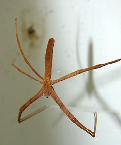
Let's return to the example, in which the feeding habits of two-species of net-casting spiders are studied. The species, the deinopis and menneus, coexist in eastern Australia. The following summary statistics were obtained on the size, in millimeters, of the prey of the two species:

Adult DEINOPIS	Adult MENNEUS
$n$ = 10	$m$ = 10
$\bar{x}$ = 10.26 mm	$\bar{y}$ = 9.02 mm
${s^2_X}$= $(2.51)^2$	${s^2_Y}$ = $(1.90)^2$

Estimate, with 95% confidence, the ratio of the two population variances.

Answer

In order to estimate the ratio of the two population variances, we need to obtain two F-values from the F-table, namely:

$F_{0.025}(9,9)=4.03$ and $F_{0.975}(9,9)=\dfrac{1}{F_{0.025}(9,9)}=\dfrac{1}{4.03}$

Then, the 95% confidence interval for the ratio of the two population variances is:

$\dfrac{1}{4.03} \left(\dfrac{2.51^2}{1.90^2}\right) \leq \dfrac{\sigma^2_X}{\sigma^2_Y} \leq 4.03 \left(\dfrac{2.51^2}{1.90^2}\right)$

Simplifying, we get:

$0.433\leq \dfrac{\sigma^2_X}{\sigma^2_Y} \leq7.033$

That is, we can be 95% confident that the ratio of the two population variances is between 0.433 and 7.033. (Because the interval contains the value 1, we cannot conclude that the population variances differ.)

Now that we've spent two pages learning confidence intervals for variances, I have a confession to make. It turns out that confidence intervals for variances have generally lost favor with statisticians, because they are not very accurate when the data are not normally distributed. In that case, we say they are "sensitive" to the normality assumption, or the intervals are "not robust."

Minitab^®

Using Minitab

Confidence Interval for Two Variances

Under the Stat menu, select Basic Statistics, and then select 2 Variances...:
In the pop-up window that appears, in the box labeled Data, select Sample standard deviations (or alternatively Sample variances). In the box labeled Sample size, type in the size n of the First sample and m of the Second sample. In the box labeled Standard deviation, type in the sample standard deviations for the First and Second samples:
Click on the button labeled Options... In the pop-up window that appears, specify the confidence level, and in the box labeled Alternative, select not equal.

Then, click on OK to return to the main pop-up window.
Then, upon clicking OK on the main pop-up window, the output should appear in the Session window:

Test and CI for Two Variances

Method

Null hypothesis                Sigma (1) / Sigma (2) = 1
Alternative hypothesis    Sigma (1) / Sigma (2) not = 1
Significance level             Alpha = 0.05

Statistics

Sample	N	StDev	Variance
1	10	2.510	6.300
2	10	1.900	3.610

Ratio of standard deviations = 1.321
Ratio of variances = 1.745

95% Confidence Intervals

Distribution of Data	CI for StDev Ratio	CI for Variance Ratio
Normal	(0.685, 2.651)	(0.433, 7.026)

Lesson 5: Confidence Intervals for Proportions

On to yet more population parameters! In this lesson, we derive formulas for $(1-\alpha)100\%$ confidence intervals for:

a population proportion $p$
the difference in two population proportions, that is, $p_1-p_2$

5.1 - One Proportion

Example 5-1

The article titled "Poll shows increasing concern, little impact with malpractice crisis" in the February 20th, 2003 issue of the Centre Daily Times reported that $n=418$ Pennsylvanians were surveyed about their opinions about insurance rates. Of the 418 surveyed, $Y=280$ blamed rising insurance rates on large court settlements against doctors. That is, the sample proportion is:

$\hat{p}=\dfrac{280}{418}=0.67$

Use this sample proportion to estimate, with 95% confidence, the parameter $p$, that is, the proportion of all Pennsylvanians who blame rising insurance rates on large court settlements against doctors.

Answer

We'll need some theory before we can really find the confidence interval for the population proportion $p$, but we can at least get the ball rolling here. Let:

$X_i=1$, if randomly selected Pennsylvanian $i$ blames rising insurance rates on large court settlements against doctors
$X_i=0$, if randomly selected Pennsylvanian $i$ does not blame rising insurance rates on large court settlements against doctors

Then, the number of Pennsylvanians in the random sample who blame rising insurance rates on large court settlements against doctors is:

$Y=\sum\limits_{i=1}^{418} X_i=280$

and therefore, the proportion of Pennsylvanians in the random sample who blame rising insurance rates on large court settlements against doctors is:

$\hat{p}=\dfrac{\sum_{i=1}^n X_i}{n}=\dfrac{280}{418}=0.67$

Well, alright, so we're right back where we started, as we basically just repeated what we were given. Well, not quite! That most recent sample proportion was written in order to emphasize the fact that a sample proportion can really be thought of as just a sample average (of 0 and 1 data):

$\hat{p}=\frac{\sum_{i=1}^n X_i }{n}=0.67$

Ohhhhh... so that means we can use what we know about the sampling distribution of $\bar{X}$ to derive a confidence interval for the population proportion $p$.

Let's jump ahead and state the result, and then we'll step back and prove it.

Theorem

For large random samples, a $(1-\alpha)100\%$ confidence interval for a population proportion $p$ is:

$\hat{p}-z_{\alpha/2}\sqrt{\dfrac{\hat{p}(1-\hat{p})}{n}} \leq p \leq \hat{p}+z_{\alpha/2}\sqrt{\dfrac{\hat{p}(1-\hat{p})}{n}}$

Proof

Okay, so where were we? That's right... we were talking about the the sampling distribution of $\bar{X}$. Well, we know that the Central Limit Theorem tells us, for large $n$, that:

$Z=\dfrac{\bar{X}-\mu}{\sigma/\sqrt{n}}$

follows, at least approximately, a standard normal distribution $N(0,1)$. Now, because:

$Z=\dfrac{\bar{x}-\mu}{\sigma/\sqrt{n}} \\ \bar{x}=\hat{p}, \qquad \mu=E(X_i)=p, \qquad \sigma^2=\text{Var}(X_i)=p(1-p)\\ \Rightarrow Z=\frac{\hat{p}-p}{\sqrt{\frac{p(1-p)}{n}}}$

that implies, for large $n$, that:

$Z=\dfrac{\hat{p}-p}{\sqrt{\dfrac{p(1-p)}{n}}}$

also follows, at least approximately, a standard normal distribution $N(0,1)$. So, we can do our usual trick of starting with a probability statement:

$P \left[-z_{\alpha/2}\leq \dfrac{\hat{p}-p}{\sqrt{\dfrac{p(1-p)}{n}}} \leq z_{\alpha/2}\right] \approx 1-\alpha$

and manipulating the quantity inside the parentheses:

$-z_{\alpha/2}\leq \dfrac{\hat{p}-p}{\sqrt{\dfrac{p(1-p)}{n}}} \leq z_{\alpha/2} $

to get the formula for a $(1-\alpha)100\%$ confidence interval for $p$. Multiplying through the inequality by the quantity in the denominator, we get:

$-z_{\alpha/2} \sqrt{\dfrac{p(1-p)}{n}} \leq \hat{p}-p \leq z_{\alpha/2} \sqrt{\dfrac{p(1-p)}{n}}$

Subtracting through the inequality by $\hat{p}$, we get:

$-\hat{p}-z_{\alpha/2} \sqrt{\dfrac{p(1-p)}{n}} \leq -p \leq -\hat{p}+z_{\alpha/2}\sqrt{\dfrac{p(1-p)}{n}}$

And, upon dividing through by −1, and thereby reversing the inequality, we get the claimed $(1-\alpha)100\%$ confidence interval for $p$:

$\hat{p}-z_{\alpha/2} \sqrt{\dfrac{p(1-p)}{n}} \leq p \leq \hat{p}+z_{\alpha/2} \sqrt{\dfrac{p(1-p)}{n}}$

Oooops! What's wrong with that confidence interval? Hmmmm.... it appears that we need to know the population proportion $p$ in order to estimate the population proportion $p$.

That's clearly not going to work. What's the logical thing to do? That's right... replace the population proportions ($p$) that appear in the endpoints of the interval with sample proportions ($\hat{p}$) to get an (approximate) $(1-\alpha)100\%$ confidence interval for $p$:

$\hat{p}-z_{\alpha/2} \sqrt{\dfrac{\hat{p}(1-\hat{p})}{n}} \leq p \leq \hat{p}+z_{\alpha/2} \sqrt{\dfrac{\hat{p}(1-\hat{p})}{n}}$

as was to be proved!

Now that we have that theory behind us, let's return to our example!

Example 5-1 (continued)

The article titled "Poll shows increasing concern, little impact with malpractice crisis" in the February 20th issue of the Centre Daily Times reported that $n=418$ Pennsylvanians were surveyed about their opinions about insurance rates. Of the 418 surveyed, $Y=280$ blamed rising insurance rates on large court settlements against doctors. That is, the sample proportion is:

$\hat{p}=\dfrac{280}{418}=0.67$

Use this sample proportion to estimate, with 95% confidence, the parameter $p$, that is, the proportion of all Pennsylvanians who blame rising insurance rates on large court settlements against doctors.

Answer

Plugging $n=418$, a sample proportion of 0.67, and $z_{0.025}=1.96$ into the formula for a 95% confidence interval for $p$, we get:

$0.67 \pm 1.96\sqrt{\dfrac{0.67(1-0.67)}{418}}$

which, upon simplifying, is:

$0.67 \pm 0.045$

which equals:

$(0.625,0.715)$

We can be 95% confident that between 62.5% and 71.5% of all Pennsylvanians blame rising insurance rates on large court settlements against doctors.

Minitab^®

Using Minitab

As is always the case, you will probably want to calculate your confidence intervals for proportions using statistical software, such as Minitab, rather than doing it by way of formula and calculator. It's easy enough to calculate the (approximate) confidence interval for $p$ using Minitab:

Under the Stat menu, select Basic Statistics, and then 1 Proportion...:
In the pop-up window that appears, select Summarized data, and enter the Number of events of interest that occurred, as well as the Number of trials (that is, the sample size n):
Click on the Options... button. If you want a confidence level that differs from the default 95.0 level, specify the desired level in the box labeled Confidence level. Click on the box labeled Use test and interval based on normal distribution. Select OK.
Select OK again on the primary pop-up window. The output should appear in the Session window:

Test and CI for One Proportion

Sample	X	N	Sample p	95% CI
1	280	418	0.669856	(0.624775, 0.714938)

Using the normal approximation.

Notes

Step 1
Our calculated margin of error is 4.5%:

$0.67\pm \mathbf{0.045}$

But, if you go back and take a look at the original article ("Poll shows increasing concern, little impact with malpractice crisis"), the newspaper's reported margin of error is 4.8%. What happened here? Why the difference? One possibility is that the newspaper was taking advantage of what is known about the maximum value of:

$\hat{p}(1-\hat{p})$

That is, the maximum value can be shown to be $\frac{1}{4}$, as demonstrated here:

If we graph the function $\hat{p}(1-\hat{p})$, it looks (roughly) like this:

We need to find the peak value, that is, the value marked by the red question mark (?). We can do that, of course, by taking the derivative of the function with respect to $\hat{p}$, setting to 0, and solving for $\hat{p}$. Taking the derivative and setting to 0, we get:

$\dfrac{d(\hat{p}-\hat{p}^2)}{d\hat{p}}=1-2\hat{p}\equiv 0$

And, solving for $\hat{p}$, we get:

$\hat{p}=\dfrac{1}{2}$

Well, that's encouraging... the point at which we've determined that the maximum occurs at least agrees with our graph! Now, what is the value of the function $\hat{p}(1-\hat{p})$ when $\hat{p}=\dfrac{1}{2}$? Well, it is:

$\hat{p}-\hat{p}^2=\dfrac{1}{2}-\left(\dfrac{1}{2}\right)^2=\dfrac{1}{2}-\dfrac{1}{4}=\dfrac{1}{4}$

as was claimed.

Because the maximum value of $\hat{p}(1-\hat{p})$ can be shown to be $\frac{1}{4}$, the largest the margin of error can be for a 95% confidence interval based on a sample size of $n=418$ is:

$1.96\sqrt{\dfrac{\frac{1}{2}(1-\frac{1}{2})}{418}} \approx 2\sqrt{\dfrac{1}{4}} \sqrt{\dfrac{1}{418}}=0.0489$

Aha! First, that 95% margin of error looks eerily similar to the margin of error claimed by the newspaper. And second, that margin of error makes it look as if we can generalize a bit. Did you notice how we've reduced the 95% margin of error to an (approximate) function of the sample size $n$? In general, a 95% margin of error can be approximated by:

$\dfrac{1}{\sqrt{n}}$

Here's what that approximate 95% margin of error would like for various sample sizes $n$:
$n$ 25 64 100 900 1600

95% ME 0.20 0.125 0.10 0.033 0.025

By the way, it is of course entirely possible that the reported margin of error was not determined using the approximate 95% margin of error, as suggested above. It is feasible that the study's authors instead used a higher confidence level, or alternatively calculated the confidence interval using exact methods rather than the normal approximation.
Step 2
The approximate confidence interval for $p$ that we derived above works well if the following two conditions hold simultaneously:
- $np=\text{ the number of expected successes }\ge 5$
- $n(1-p)=\text{ the number of expected failures }\ge 5$

\(n\)	25	64	100	900	1600
95% ME	0.20	0.125	0.10	0.033	0.025

5.2 - Two Proportions

Example 5-2

Let's start our exploration of finding a confidence interval for the difference in two proportions by way of an example.

What is the prevalence of anemia in developing countries?

	African Women	Women from Americas
Sample size	2100	1900
Number with anemia	840	323
Sample proportion	$\dfrac{840}{2100}=0.40$	$\dfrac{323}{1900}=0.17$

Find a 95% confidence interval for the difference in proportions of all African women with anemia and all women from the Americas with anemia.

Answer

Let's start by simply defining some notation. Let:

$n_1$ = the number of African women sampled = 2100
$n_2$ = the number of women from the Americas sampled = 1900
$y_1$ = the number of African women with anemia = 840
$y_2$ = the number of women from the Americas with anemia = 323

Based on these data, we can calculate two sample proportions. The proportion of African women sampled who have anemia is:

$\hat{p}_1=\dfrac{840}{2100}=0.40$

And the proportion of women from the Americas sampled who have anemia is:

$\hat{p}_2=\dfrac{323}{1900}=0.17$

Now, letting:

$p_1$ = the proportion of all African women with anemia
$p_2$ = the proportion of all women from the Americas with anemia

we are then interested in finding a 95% confidence interval for $p_1-p_2$, the difference in the two population proportions. We need to derive a formula for the confidence interval before we can actually calculate it!

Theorem

For large random samples, an (approximate) $(1-\alpha)100\%$ confidence interval for $p_1-p_2$, the difference in two population proportions, is:

$(\hat{p}_1-\hat{p}_2)\pm z_{\alpha/2} \sqrt{\dfrac{\hat{p}_1(1-\hat{p}_1)}{n_1}+\dfrac{\hat{p}_2(1-\hat{p}_2)}{n_2}}$

Proof

Let's start with what we know from previous work, namely:

$\hat{p}_1=\dfrac{Y_1}{n_1} \sim N\left(p_1,\dfrac{p_1(1-p_1)}{n_1}\right)$ and $\hat{p}_2=\dfrac{Y_2}{n_2} \sim N\left(p_2,\dfrac{p_2(1-p_2)}{n_2}\right)$

By independence, therefore:

$(\hat{p}_1-\hat{p}_2) \sim N\left(p_1-p_2,\dfrac{p_1(1-p_1)}{n_1}+\dfrac{p_2(1-p_2)}{n_2}\right)$

Now, it's just a matter of transforming the inside of the typical probability statement:

$P\left[-z_{\alpha/2} \leq \dfrac{(\hat{p}_1-\hat{p}_2)-(p_1-p_2)}{\sqrt{\dfrac{p_1(1-p_1)}{n_1}+\dfrac{p_2(1-p_2)}{n_2}}} \leq z_{\alpha/2} \right] \approx 1-\alpha$

That is, we start with this:

$-z_{\alpha/2} \leq \dfrac{(\hat{p}_1-\hat{p}_2)-(p_1-p_2)}{\sqrt{\dfrac{p_1(1-p_1)}{n_1}+\dfrac{p_2(1-p_2)}{n_2}}} \leq z_{\alpha/2}$

Multiplying through the inequality by the quantity in the denominator, we get:

$-z_{\alpha/2}\sqrt{\dfrac{p_1(1-p_1)}{n_1}+\dfrac{p_2(1-p_2)}{n_2}}\leq (\hat{p}_1-\hat{p}_2)-(p_1-p_2) \leq z_{\alpha/2}\sqrt{\dfrac{p_1(1-p_1)}{n_1}+\dfrac{p_2(1-p_2)}{n_2}}$

Subtracting through the inequality by $\hat{p}_1-\hat{p}_2$, we get:

$-(\hat{p}_1-\hat{p}_2)-z_{\alpha/2}\sqrt{\dfrac{p_1(1-p_1)}{n_1}+\dfrac{p_2(1-p_2)}{n_2}}\leq -(p_1-p_2) \leq -(\hat{p}_1-\hat{p}_2)+z_{\alpha/2}\sqrt{\dfrac{p_1(1-p_1)}{n_1}+\dfrac{p_2(1-p_2)}{n_2}}$

And finally, dividing through the inequality by −1, and rearranging the inequalities, we get our confidence interval:

$(\hat{p}_1-\hat{p}_2)-z_{\alpha/2}\sqrt{\dfrac{p_1(1-p_1)}{n_1}+\dfrac{p_2(1-p_2)}{n_2}}\leq p_1-p_2 \leq (\hat{p}_1-\hat{p}_2)+z_{\alpha/2}\sqrt{\dfrac{p_1(1-p_1)}{n_1}+\dfrac{p_2(1-p_2)}{n_2}}$

Ooooppps again! What's wrong with the interval? That's right... we need to know the two population proportions in order the estimate the difference in the population proportions!!

That clearly won't work! We can again solve the problem by putting some hats on those population proportions! Doing so, we get the (approximate) $(1-\alpha)100\%$ confidence interval for $p_1-p_2$:

$(\hat{p}_1-\hat{p}_2)-z_{\alpha/2}\sqrt{\dfrac{\hat{p}_1(1-\hat{p}_1)}{n_1}+\dfrac{\hat{p}_2(1-\hat{p}_2)}{n_2}}\leq p_1-p_2 \leq (\hat{p}_1-\hat{p}_2)+z_{\alpha/2}\sqrt{\dfrac{\hat{p}_1(1-\hat{p}_1)}{n_1}+\dfrac{\hat{p}_2(1-\hat{p}_2)}{n_2}}$

as claimed.

Example 5-2 (continued)

What is the prevalence of anemia in developing countries?

	African Women	Women from Americas
Sample size	2100	1900
Number with anemia	840	323
Sample proportion	$\dfrac{840}{2100}=0.40$	$\dfrac{323}{1900}=0.17$

Find a 95% confidence interval for the difference in proportions of all African women with anemia and all women from the Americas with anemia.

Substituting in the numbers that we know into the formula for a 95% confidence interval for $p_1-p_2$, we get:

$(0.40-0.17)\pm 1.96 \sqrt{\dfrac{0.40(0.60)}{2100}+\dfrac{0.17(0.83)}{1900}}$

which simplifies to:

$0.23\pm 0.027=(0.203, 0.257)$

We can be 95% confident that there are between 20.3% and 25.7% more African women with anemia than women from the Americas with anemia.

Example 5-3

A social experiment conducted in 1962 involved $n=123$ three- and four-year-old children from poverty-level families in Ypsilanti, Michigan. The children were randomly assigned either to:

A treatment group receiving two years of preschool instruction
A control group receiving no preschool instruction.

The participants were followed into their adult years. Here is a summary of the data:

	Arrested for some crime
	Yes	No
Control	32	30
Preschool	19	42

Find a 95% confidence interval for $p_1-p_2$, the difference in the two population proportions.

Answer

Of the $n_1=62$ children serving as the control group, 32 were later arrested for some crime, yielding a sample proportion of:

$\hat{p}_1=0.516$

And, of the $n_2=61$ children receiving preschool instruction, 19 were later arrested for some crime, yielding a sample proportion of:

$\hat{p}_2=0.311$

A 95% confidence interval for $p_1-p_2$ is therefore:

$(0.516-0.311)\pm 1.96\sqrt{\dfrac{0.516(0.484)}{62}+\dfrac{0.311(0.689)}{61}}$

which simplifies to:

$0.205\pm 0.170=(0.035, 0.375)$

We can be 95% confident that between 3.5% and 37.5% more children not having attended preschool were arrested for a crime by age 19 than children who had received preschool instruction.

Minitab^®

Using Minitab

Yes, Minitab will calculate a confidence interval for the difference in two population proportions for you. To do so:

Under the Stat menu, select Basic Statistics, and then select 2 Proportions...:
In the pop-up window that appears, select Summarized data, and enter the Number of events, as well as the Number of Trials (that is, the sample sizes $n_i$) for each of two groups (First and Second) of interest:
Select OK. The output should appear in the Session window:

Sample	X	N	Sample p
1	32	62	0.516129
2	19	61	0.311475

Difference = p (1) - p (2)
Estimate for difference: 0.204654
95% CI for difference: (0.0344211, 0.374886)
Test for difference = 0 (vs not =0): Z = 2.36 P-Value = 0.018

Fisher's exact test: P-Value = 0.028

Lesson 6: Sample Size

Overview

So far, in this section, we have focused on using a random sample of size $n$ to find an interval estimate for a variety of population parameters, including a mean $\mu$, a proportion $p$, and a standard deviation $\sigma$. In none of our discussions did we talk about how large a sample should be in order to ensure that the interval estimate we obtain is narrow enough to be worthwhile. That's what we'll do in this lesson!

Objectives

Upon completion of this lesson, you should be able to:

derive a formula for the sample size, $n$, necessary for estimating the population mean $\mu$
derive a formula for the sample size, $n$, necessary for estimating a proportion $p$ for a large population
derive a formula for the sample size, $n$, necessary for estimating a proportion $p$ for a small, finite population

The methods that we use here in deriving the formulas could be easily applied to the estimation of other population parameters as well.

6.1 - Estimating a Mean

Example 6.1

A researcher wants to estimate $\mu$, the mean systolic blood pressure of adult Americans, with 95% confidence and error $\epsilon$ no larger than 3 mm Hg. How many adult Americans, $n$, should the researcher randomly sample to achieve her estimation goal?

Answer

The researcher's goal is to estimate $\mu$ so that the error is no larger than 3 mm Hg. (By the way, $\epsilon$ is typically called the maximum error of the estimate.) That is, her goal is to calculate a 95% confidence interval such that:

$\bar{x}\pm \epsilon=\bar{x}\pm 3$

Now, we know the formula for a $(1-\alpha)100\%$ confidence interval for a population mean $\mu$ is:

$\bar{x}\pm t_{\alpha/2,n-1}\left(\dfrac{s}{\sqrt{n}}\right)$

So, it seems that a reasonable way to proceed would be to equate the terms appearing after each of the above $\pm$ signs, and solve for $n$. That is, equate:

$\epsilon=t_{\alpha/2,n-1}\left(\dfrac{s}{\sqrt{n}}\right)$

and solve for $n$. Multiplying through by the square root of $n$, we get:

$\epsilon \sqrt{n}=t_{\alpha/2,n-1}(s)$

And, dividing through by $\epsilon$ and squaring both sides, we get:

$n=\dfrac{(t_{\alpha/2,n-1})^2 s^2}{\epsilon^2}$

Now, what's wrong with the formula we derived? Well... the $t$-value on the right side of the equation depends on $n$.

That's not particularly helpful given that we are trying to find $n$! We can solve that problem by simply replacing the $t$-value that depends on $n$ with a $Z$-value that doesn't. After all, you might recall that as $n$ increases, the $t$-distribution approaches the standard normal distribution. Doing so, we get:

$n \approx \dfrac{(z^2_{\alpha/2})s^2}{\epsilon^2}$

Before we make the calculation for our particular example, let's take a step back and summarize what we have just learned.

Estimating a population mean $\mu$

The sample size necessary for estimating a population mean $\mu$ with $(1-\alpha)100\%$ confidence and error no larger than $\epsilon$ is:

$n = \dfrac{(z^2_{\alpha/2})s^2}{\epsilon^2}$

Typically, the hardest part of determining the necessary sample size is finding $s^2$, that is, a decent estimate of the population variance. There are a few ways of obtaining $s^2$.

Ways to Determine $s^2$

You can often get $s^2$, an estimate of the population variance from the scientific literature. After all, scientific research is typically not done in a vacuum. That is, what one researcher is studying and reporting in scientific journals is typically also studied and reported by several other researchers in various locations around the world. If you're in need of an estimate of the variance of the front leg length of red-eyed tree frogs, you'll probably be able to find it in a research paper reported in some scientific journal.
You can often get $s^2$, an estimate of the population variance by conducting a small pilot study on 5-10 people (or trees or snakes or... whatever you're measuring).
You can often get $s^2$, an estimate of the population variance by using what we know about the Empirical Rule, which states that we can expect 95% of the observations to fall in the interval:

$\bar{x}\pm 2s$

Here's a picture that illustrates how this part of the Empirical Rule can help us determine a reasonable value of $s$:

That is, we could define the range of values as that which captures 95% of the measurements. If we do that, then we can work backwards to see that s can be determined by dividing the range by 4. That is:

$s=\dfrac{Range}{4}=\dfrac{Max-Min}{4}$

When statisticians use the Empirical Rule to help a researcher arrive at a reasonable value of $s$, they almost always use the above formula. That said, there may be occasion in which it is worthwhile using another part of the Empirical Rule, namely that we can expect 99.7% of the observations to fall in the interval:

$\bar{x}\pm 3s$

Here's a picture that illustrates how this part of the Empirical Rule can help us determine a reasonable value of $s$:

In this case, we could define the range of values as that which captures 99.7% of the measurements. If we do that, then we can work backwards to see that $s$ can be determined by dividing the range by 6. That is:

$s=\dfrac{Range}{6}=\dfrac{Max-Min}{6}$

Example 6-1 (Continued)

A researcher wants to estimate $\mu$, the mean systolic blood pressure of adult Americans, with 95% confidence and error $\epsilon$ no larger than 3 mm Hg. How many adult Americans, $n$, should the researcher randomly sample to achieve her estimation goal?

Answer

If the maximum error $\epsilon$ is 3, and the sample variance is $s^2=10^2$, we need:

$n=\dfrac{(1.96)^2(10)^2}{3^2}=42.7$

or 43 people to estimate $\mu$ with 95% confidence. In general, when making sample size calculations such at this one, it is a good idea to change all of the factors to see what the "cost" in sample size is for achieving certain errors $\epsilon$ and confidence levels $(1-\alpha)$. Doing that here, we get:

$s^2 = 10^2$	$ \epsilon $= 1	$ \epsilon $= 3	$ \epsilon $= 5
90% $(z_{0.05} = 1.645)$	271	31	11
95% $(z_{0.025} = 1.96)$	385	43	16
99% $(z_{0.005} = 2.576)$	664	74	27

We can also change the estimate of the variance. For example, if we change the sample variance to $s^2=8^2$, then the necessary sample sizes for various errors $\epsilon$ and confidence levels $(1-\alpha)$ become:

$s^2 = 8^2$	$ \epsilon $= 1	$ \epsilon $= 3	$ \epsilon $= 5
90% $(z_{0.05} = 1.645)$	174	20	7
95% $(z_{0.025} = 1.96)$	246	28	10
99% $(z_{0.005} = 2.576)$	425	48	17

Factors Affecting the Sample Size

If we take a look back at the formula for the sample size:

$n =\dfrac{(z^2_{\alpha/2})s^2}{\epsilon^2}$

we can make some generalizations about how each of three factors, namely the standard deviation s, the confidence level $(1-\alpha)100\%$, and the error $\epsilon$, affect the necessary sample size.

As the confidence level $(1-\alpha)100\%$ increases, the necessary sample size increases. That's because as the confidence level increases, the $Z$-value, which appears in the numerator of the formula, increases. Again, you can see an example of this generalization from some of the numbers generated in that last example:

As the error $\epsilon$ decreases, the necessary sample size $n$ increases. That's because the error $epsilon$ term appears in the denominator. You can see an example of this generalization from some of the numbers generated in that last example:

Hover over the icon to see further explanation

$s^2 = 10^2$	$ \epsilon $= 1	$ \epsilon $= 3	$ \epsilon $= 5
90% $(z_{0.05} = 1.645)$	271	31	11
95% $(z_{0.025} = 1.96)$	385	43	16
99% $(z_{0.005} = 2.576)$	664	74	27

As the confidence level $(1-\alpha)100\%$ increases, the necessary sample size increases. That's because as the confidence level increases, the $Z$-value, which appears in the numerator of the formula, increases. Again, you can see an example of this generalization from some of the numbers generated in that last example:

Hover over the icon to see further explanation

$s^2 = 8^2$	$ \epsilon $= 1	$ \epsilon $= 3	$ \epsilon $= 5
90% $(z_{0.05} = 1.645)$	174	20	7
95% $(z_{0.025} = 1.96)$	246	28	10
99% $(z_{0.005} = 2.576)$	425	48	17

As the sample standard deviation $s$ increases, the necessary sample size increases. That's because the standard deviation s appears in the numerator of the formula. Again, you can see an example of this generalization from some of the numbers generated in that last example:

$s^2 = 10^2$	$ \epsilon $= 1	$ \epsilon $= 3	$ \epsilon $= 5
90% $(z_{0.05} = 1.645)$	271	31	11
95% $(z_{0.025} = 1.96)$	385	43	16
99% $(z_{0.005} = 2.576)$	664	74	27

$s^2 = 8^2$	$ \epsilon $= 1	$ \epsilon $= 3	$ \epsilon $= 5
90% $(z_{0.05} = 1.645)$	174	20	7
95% $(z_{0.025} = 1.96)$	246	28	10
99% $(z_{0.005} = 2.576)$	425	48	17

6.2 - Estimating a Proportion for a Large Population

Example 6-2

A pollster wants to estimate $p$, the true proportion of all Americans favoring the Democratic candidate with 95% confidence and error $\epsilon$ no larger than 0.03.

How many people should he randomly sample to achieve his goals?

Answer

We'll tackle this problem just as we did for finding the sample size necessary to estimate a population mean. First, note that the pollster's goal is to estimate the population proportion $p$ so that the error is no larger than 0.03. That is, the goal is to calculate a 95% confidence interval such that:

$\hat{p}\pm \epsilon=\hat{p}\pm 0.03$

But, we know the formula for a $(1-\alpha)100\%$ confidence interval for a population proportion is:

$\hat{p}\pm z_{\alpha/2}\sqrt{\dfrac{\hat{p}(1-\hat{p})}{n}}$

So, just as we did on the previous page, we'll proceed by equating the terms appearing after each of the above $\pm$ signs, and solve for $n$. That is, equate:

$\epsilon=z_{\alpha/2}\sqrt{\dfrac{\hat{p}(1-\hat{p})}{n}}$

and solve for $n$. Multiplying through by the square root of $n$, we get:

$\epsilon \sqrt{n}=z_{\alpha/2}\sqrt{\hat{p}(1-\hat{p})}$

And, dividing through by $\epsilon$ and squaring both sides, we get:

$n=\dfrac{z^2_{\alpha/2}\hat{p}(1-\hat{p})}{\epsilon^2}$

Again, before we make the calculation for our particular example, let's take a step back and summarize the formula that we have just derived.

Estimating a population proportion $p$

The sample size necessary for estimating a population proportion $p$ of a large population with ((1-\alpha)100\%\) confidence and error no larger than $\epsilon$ is:

$n=\dfrac{z^2_{\alpha/2}\hat{p}(1-\hat{p})}{\epsilon^2}$

Just as we needed to have a decent estimate, $s^2$, of the population variance when calculating the sample size necessary for estimating a population mean $\mu$, we need to have a good estimate, $\hat{p}$, of the population proportion when calculating the sample size necessary for estimating a population proportion $p$. Strange, I know... but there are at least two ways out of this conundrum.

Ways to Determine $\hat{p}(1-\hat{p})$

You can use your prior knowledge (previous polls, perhaps?) about $\hat{p}$.
You can set $\hat{p}(1-\hat{p})=\dfrac{1}{4}$ , its maximum when $\hat{p}=\dfrac{1}{2}$

Example 6-2 (Continued)

A pollster wants to estimate $p$, the true proportion of all Americans favoring the Democratic candidate with 95% confidence and error $\epsilon$ no larger than 0.03.

How many people should he randomly sample to achieve his goals?

Answer

If the maximum error $\epsilon$ is 0.03, and the sample proportion is 0.8, we need to survey:

$n=\dfrac{(1.96)^2(0.8)(0.2)}{0.03^2}=682.95$

or 683 people to estimate $p$ with 95% confidence. Again, when making sample size calculations such at this one, it is a good idea to change all of the factors to see what the "cost" is in sample size for achieving certain errors $\epsilon$ and confidence levels $(1-\alpha)$. Doing that here, we get:

$ \hat{p} = 0.8$	$ \epsilon $= 1	$ \epsilon $= 3	$ \epsilon $= 5
90% $(z_{0.05} = 1.645)$	4330	482	174
95% $(z_{0.025} = 1.96)$	6147	683	246
99% $(z_{0.005} = 2.576)$	10618	1180	425

We, of course, can also change the sample proportion. For example, if we change the sample proportion to 0.5, then we need to survey:

$n=\dfrac{(1.96)^2(0.5)(0.5)}{0.03^2}=1067.1$

or 1068 people to estimate $p$ with 95% confidence. The two calculations in this example illustrate how useful it is to have some idea of the magnitude of the sample proportion. In one case, if the proportion is close to 0.80, then we'd need as few as 680 people. On the other hand, if the proportion is close to 0.50, then we'd need as many as 1070 people. That difference in necessary sample size sure argues for a small pilot study in advance of the larger survey.

By the way, just as we did for the case in which the sample proportion was 0.8, we can change the factors to see what the "cost" is in sample size for achieving certain errors $\epsilon$ and confidence levels $(1-\alpha)$. Doing that here, we get:

$ \hat{p} = 0.5$	$ \epsilon $= 1	$ \epsilon $= 3	$ \epsilon $= 5
90% $(z_{0.05} = 1.645)$	6766	752	271
95% $(z_{0.025} = 1.96)$	9604	1068	385
99% $(z_{0.005} = 2.576)$	16590	1844	664

6.3 - Estimating a Proportion for a Small, Finite Population

The methods of the last page, in which we derived a formula for the sample size necessary for estimating a population proportion $p$ work just fine when the population in question is very large. When we have smaller, finite populations, however, such as the students in a high school or the residents of a small town, the formula we derived previously requires a slight modification. Let's start, as usual, by taking a look at an example.

Example 6-3

A researcher is studying the population of a small town in India of $N=2000$ people. She's interested in estimating $p$ for several yes/no questions on a survey.

How many people $n$ does she have to randomly sample (without replacement) to ensure that her estimates $\hat{p}$ are within $\epsilon=0.04$ of the true proportions $p$?

Answer

We can't even begin to address the answer to this question until we derive a confidence interval for a proportion for a small, finite population!

Theorem

An approximate ($(1-\alpha)100\%$ confidence interval for a proportion $p$ of a small population is:

$\hat{p}\pm z_{\alpha/2}\sqrt{\dfrac{\hat{p}(1-\hat{p})}{n} \cdot \dfrac{N-n}{N-1}}$

Proof

We'll use the example above, where possible, to make the proof more concrete. Suppose we take a random sample, $X_1, X_2, \ldots, X_n$, without replacement, of size $n$ from a population of size $N$. In the case of the example, $N=2000$. Suppose also, unknown to us, that for a particular survey question there are $N_1$ respondents who would respond "yes" to the question, and therefore $N-N_1$ respondents who would respond "no." That is, our small finite population looks like this:

If that's the case, the true proportion (but unknown to us) of yes respondents is:

$p=P(Yes)=\dfrac{N_1}{N}$

while the true proportion (but unknown to us) of no respondents is:

$1-p=P(No)=1-\dfrac{N_1}{N}=\dfrac{N-N_1}{N}$

Now, let $X$ denote the number of respondents in the sample who say yes, so that:

$X=\sum\limits_{i=1}^n X_i$

if $X_i=1$ if respondent $i$ answers yes, and $X_i=0$ if respondent $i$ answers no. Then, the proportion in the sample who say yes is:

$\hat{p}=\dfrac{\sum\limits_{i=1}^n X_i}{n}$

Then, $X=\sum\limits_{i=1}^n X_i$ is a hypergeometric random variable with mean:

$E(X)=n\dfrac{N_1}{N}=np$

and variance: $$Var(X)=n{N_1\over N}\left(1-{N_1\over N}\right) \left({N-n\over N-1}\right)=np(1-p)\left({N-n\over N-1}\right)$$

It follows that $\hat{p}=X/n$ has mean $E(\hat{p})=p$ and variance:

$Var(\hat{p})=\dfrac{p(1-p)}{n}\left(\dfrac{N-n}{N-1}\right)$

Then, the Central Limit Theorem tells us that:

$\dfrac{\hat{p}-p}{\sqrt{\dfrac{p(1-p)}{n} \left(\dfrac{N-n}{N-1}\right) }}$

follows an approximate standard normal distribution. Now, it's just a matter of doing the typical confidence interval derivation, in which we start with a probability statement, manipulate the quantity inside the parentheses, and substitute sample estimates where necessary. We've done that a number of times now, so skipping all of the details here, we get that an approximate $(1-\alpha)100\%$ confidence interval for $p$ of a small population is:

$\hat{p}\pm z_{\alpha/2}\sqrt{\dfrac{\hat{p}(1-\hat{p})}{n} \cdot \dfrac{N-n}{N-1}}$

By the way, it is worthwhile noting that if the sample $n$ is much smaller than the population size $N$, that is, if $n<<N$, then:

$\dfrac{N-n}{N-1}\approx 1$

and the confidence interval for $p$ of a small population becomes quite similar to the confidence interval for $p$ of a large population:

$\hat{p}\pm z_{\alpha/2}\sqrt{\dfrac{\hat{p}(1-\hat{p})}{n}}$

Example 6-3 (continued)

A researcher is studying the population of a small town in India of $N=2000$ people. She's interested in estimating $p$ for several yes/no questions on a survey.

How many people $n$ does she have to randomly sample (without replacement) to ensure that her estimates $\hat{p}$ are within $\epsilon=0.04$ of the true proportion $p$?

Answer

Now that we know the correct formula for the confidence interval for $p$ of a small population, we can follow the same procedure we did for determining the sample size for estimating a proportion $p$ of a large population. The researcher's goal is to estimate $p$ so that the error is no larger than 0.04. That is, the goal is to calculate a 95% confidence interval such that:

$\hat{p}\pm \epsilon=\hat{p}\pm 0.04$

Now, we know the formula for an approximate $(1-\alpha)100\%$ confidence interval for a proportion $p$ of a small population is:

$\hat{p}\pm z_{\alpha/2}\sqrt{\dfrac{\hat{p}(1-\hat{p})}{n} \cdot \dfrac{N-n}{N-1}}$

So, again, we should proceed by equating the terms appearing after each of the above $\pm$ signs, and solving for $n$. That is, equate:

$\epsilon=z_{\alpha/2}\sqrt{\dfrac{\hat{p}(1-\hat{p})}{n}\cdot \dfrac{N-n}{N-1}}$

and solve for $n$. Doing the algebra yields:

$n=\dfrac{z^2_{\alpha/2}\hat{p}(1-\hat{p})/\epsilon^2}{\dfrac{N-1}{N}+\dfrac{z^2_{\alpha/2}\hat{p}(1-\hat{p})}{N\epsilon^2}}$

That looks simply dreadful! Let's make it look a little more friendly to the eyes:

$n=\dfrac{m}{1+\dfrac{m-1}{N}}$

where $m$ is defined as the sample size necessary for estimating the proportion $p$ for a large population, that is, when a correction for the population being small and finite is not made. That is:

$m=\dfrac{z^2_{\alpha/2}\hat{p}(1-\hat{p})}{\epsilon^2}$

Now, before we make the calculation for our particular example, let's take a step back and summarize what we have just learned.

Estimating a population proportion $p$ of a small finite population

The sample size necessary for estimating a population proportion $p$ of a small finite population with $(1-\alpha)100\%$ confidence and error no larger than $\epsilon$ is:

$n=\dfrac{m}{1+\dfrac{m-1}{N}}$

where:

$m=\dfrac{z^2_{\alpha/2}\hat{p}(1-\hat{p})}{\epsilon^2}$

is the sample size necessary for estimating the proportion $p$ for a large population.

Example 6-3 (continued)

A researcher is studying the population of a small town in India of $N=2000$ people. She's interested in estimating $p$ for several yes/no questions on a survey.

How many people $n$ does she have to randomly sample (without replacement) to ensure that her estimates $\hat{p}$ are within $\epsilon=0.04$ of the true proportion $p$?

Answer

Okay, once and for all, let's calculate this very patient researcher's sample size! Because the researcher has many different questions on the survey, it would behoove her to use a sample proportion of 0.50 in her calculations. If the maximum error $\epsilon$ is 0.04, the sample proportion is 0.5, and the researcher doesn't make the finite population correction, then she needs:

$m=\dfrac{(1.96^2)(\frac{1}{4})}{0.04^2}=600.25$

or 601 people to estimate $p$ with 95% confidence. But, upon making the correction for the small, finite population, we see that the researcher really only needs:

$n=\dfrac{m}{1+\dfrac{m-1}{N}}=\dfrac{601}{1+\dfrac{601-1}{2000}}=462.3$

or 463 people to estimate $p$ with 95% confidence.

Effect of Population Size $N$

The following table illustrates how the sample size $n$ that is necessary for estimating a population proportion $p$ (with 95% confidence) is affected by the size of the population $N$. If $\hat{p}=0.5$, then the sample size $n$ is:

$ \hat{p} = 0.5$	$ \large \epsilon $= 0.01	$ \large \epsilon $= 0.03	$ \large \epsilon $= 0.05
N very large	9604	1068	385
N = 10, 000, 000	9595	1068	385
N = 1, 000, 000	9513	1067	385
N = 100, 000	8763	1057	384
N = 10, 000	4900	966	371
N = 1, 000	906	517	279

This table suggests, perhaps not surprisingly, that as the size of the population $N$ decreases, so does the necessary size $n$ of the sample.

Lesson 7: Simple Linear Regression

Overview

Simple linear regression is a way of evaluating the relationship between two continuous variables. One variable is regarded as the predictor variable, explanatory variable, or independent variable $(x)$. The other variable is regarded as the response variable, outcome variable, or dependent variable $(y)$.

For example, we might we interested in investigating the (linear?) relationship between:

heights and weights
high school grade point averages and college grade point averages
speed and gas mileage
outdoor temperature and evaporation rate
the Dow Jones industrial average and the consumer confidence index

7.1 - Types of Relationships

Before we dig into the methods of simple linear regression, we need to distinguish between two different type of relationships, namely:

deterministic relationships
statistical relationships

As we'll soon see, simple linear regression concerns statistical relationships.

Deterministic (or Functional) Relationships

A deterministic (or functional) relationship is an exact relationship between the predictor $x$ and the response $y$. Take, for instance, the conversion relationship between temperature in degrees Celsius $(C)$ and temperature in degrees Fahrenheit $(F)$. We know the relationship is:

$F=\dfrac{9}{5}C+32$

Therefore, if we know that it is 10 degrees Celsius, we also know that it is 50 degrees Fahrenheit:

$F=\dfrac{9}{5}(10)+32=50$

This is what the exact (linear) relationship between degrees Celsius and degrees Fahrenheit looks like graphically:

Other examples of deterministic relationships include the relationship between the diameter $(d)$ and circumference of a circle $(C)$:

$C=\pi \times d$

the relationship between the applied weight $(X)$ and the amount of stretch in a spring $(Y)$ (known as Hooke's Law):

$Y=\alpha+\beta X$

the relationship between the voltage applied $(V)$, the resistance $(r)$ and the current $(I)$ (known as Ohm's Law):

$I=\dfrac{V}{r}$

and, for a constant temperature, the relationship between pressure $(P)$ and volume of gas $(V)$ (known as Boyle's Law):

$P=\dfrac{\alpha}{V}$

where $\alpha$ is a known constant for each gas.

Statistical Relationships

A statistical relationship, on the other hand, is not an exact relationship. It is instead a relationship in which "trend" exists between the predictor $x$ and the response $y$, but there is also some "scatter." Here's a graph illustrating how a statistical relationship might look:

In this case, researchers investigated the relationship between the latitude (in degrees) at the center of each of the 50 U.S. states and the mortality (in deaths per 10 million) due to skin cancer in each of the 50 U.S. states. Perhaps we shouldn't be surprised to see a downward trend, but not an exact relationship, between latitude and skin cancer mortality. That is, as the latitude increases for the northern states, in which sun exposure is less prevalent and less intense, mortality due to skin cancer decreases, but not perfectly so.

Other examples of statistical relationships include:

the positive relationship between height and weight
the positive relationship between alcohol consumed and blood alcohol content
the negative relationship between vital lung capacity and pack-years of smoking
the negative relationship between driving speed and gas mileage

It is these type of less-than-perfect statistical relationships that we are interested in when we investigate the methods of simple linear regression.

7.2 - Least Squares: The Idea

Example 7-1

Before delving into the theory of least squares, let's motivate the idea behind the method of least squares by way of example.

A student was interested in quantifying the (linear) relationship between height (in inches) and weight (in pounds), so she measured the height and weight of ten randomly selected students in her class. After taking the measurements, she created the adjacent scatterplot of the obtained heights and weights. Wanting to summarize the relationship between height and weight, she eyeballed what she thought were two good lines (solid and dashed), but couldn't decide between:

$\text{weight} = −266.5 + 6.1\times \text{height}$
$\text{weight} = −331.2 + 7.1\times \text{height}$

Which is the "best fitting line"?

Answer

In order to facilitate finding the best fitting line, let's define some notation. Recalling that an experimental unit is the thing being measured (in this case, a student):

let $y_i$ denote the observed response for the $i^{th}$ experimental unit
let $x_i$ denote the predictor value for the $i^{th}$ experimental unit
let $\hat{y}_i$ denote the predicted response (or fitted value) for the $i^{th}$ experimental unit

Therefore, for the data point circled in red:

we have:

$x_i=75$ and $y_i=208$

And, using the unrounded version of the proposed line, the predicted weight of a randomly selected 75-inch tall student is:

$\hat{y}_i=-266.534+6.13758(75)=193.8$

pounds. Now, of course, the estimated line does not predict the weight of a 75-inch tall student perfectly. In this case, the prediction is 193.8 pounds, when the reality is 208 pounds. We have made an error in our prediction. That is, in using $\hat{y}_i$ to predict the actual response $y_i$ we make a prediction error (or a residual error) of size:

$e_i=y_i-\hat{y}_i$

Now, a line that fits the data well will be one for which the $n$ prediction errors (one for each of the $n$ data points — $n=10$, in this case) are as small as possible in some overall sense. This idea is called the "least squares criterion." In short, the least squares criterion tells us that in order to find the equation of the best fitting line:

$\hat{y}_i=a_1+bx_i$

we need to choose the values $a_1$ and $b$ that minimize the sum of the squared prediction errors. That is, find $a_1$ and $b$ that minimize:

$Q=\sum\limits_{i=1}^n (y_i-\hat{y}_i)^2=\sum\limits_{i=1}^n (y_i-(a_1+bx_i))^2$

So, using the least squares criterion to determine which of the two lines:

$\text{weight} = −266.5 + 6.1 \times\text{height}$
$\text{weight} = −331.2 + 7.1 \times \text{height}$

is the best fitting line, we just need to determine $Q$, the sum of the squared prediction errors for each of the two lines, and choose the line that has the smallest value of $Q$. For the dashed line, that is, for the line:

$\text{weight} = −331.2 + 7.1\times\text{height}$

here's what the work would look like:

`i`	`$ x_i $`	`$ y_i $`	`$ \hat{y_i} $`	`$ y_i -\hat{y_i} $`	`$ (y_i - \hat{y_i})^2 $`
1	64	121	123.2	-2.2	4.84
2	73	181	187.1	-6.1	37.21
3	71	156	172.9	-16.9	285.61
4	69	162	158.7	3.3	10.89
5	66	142	137.4	4.6	21.16
6	69	157	158.7	-1.7	2.89
7	75	208	201.3	6.7	44.89
8	71	169	172.9	-3.9	15.21
9	63	127	116.1	10.9	118.81
10	72	165	180.0	-15.0	225.00
					------
					766.51

The first column labeled $i$ just keeps track of the index of the data points, $i=1, 2, \ldots, 10$. The columns labeled $x_i$ and $y_i$ contain the original data points. For example, the first student measured is 64 inches tall and weighs 121 pounds. The fourth column, labeled $\hat{y}_i$, contains the predicted weight of each student. For example, the predicted weight of the first student, who is 64 inches tall, is:

$\hat{y}_1=-331.2+7.1(64)=123.2$

pounds. The fifth column contains the errors in using $\hat{y}_i$ to predict $y_i$. For the first student, the prediction error is:

$e_1=121-123.3=-2.2$

And, the last column contains the squared prediction errors. The squared prediction error for the first student is:

$e^2_1=(-2.2)^2=4.84$

By summing up the last column, that is, the column containing the squared prediction errors, we see that $Q= 766.51$ for the dashed line. Now, for the solid line, that is, for the line:

$\text{weight} = −266.5 + 6.1\times\text{height}$

here's what the work would look like:

`i`	`$ x_i $`	`$ y_i $`	`$ \hat{y_i} $`	`$ y_i -\hat{y_i} $`	`$ (y_i - \hat{y_i})^2 $`
1	64	121	126.271	-5.3	28.9
2	73	181	181.509	-0.5	0.25
3	71	156	169.234	-13.2	174.24
4	69	162	156.959	5.0	25.00
5	66	142	138.546	3.5	12.25
6	69	157	156.959	0.0	0.00
7	75	208	193.784	14.2	201.64
8	71	169	169.234	-0.2	0.04
9	63	127	120.133	6.9	47.61
10	72	165	175.371	-10.4	108.16
					------
					597.28

The calculations for each column are just as described previously. In this case, the sum of the last column, that is, the sum of the squared prediction errors for the solid line is $Q= 597.28$. Choosing the equation that minimizes $Q$, we can conclude that the solid line, that is:

$\text{weight} = −266.5 + 6.1\times\text{height}$

is the best fitting line.

In the preceding example, there's one major problem with concluding that the solid line is the best fitting line! We've only considered two possible candidates. There are, in fact, an infinite number of possible candidates for best fitting line. The approach we used above clearly won't work in practice. On the next page, we'll instead derive some formulas for the slope and the intercept for least squares regression line.

7.3 - Least Squares: The Theory

Now that we have the idea of least squares behind us, let's make the method more practical by finding a formula for the intercept $a_1$ and slope $b$. We learned that in order to find the least squares regression line, we need to minimize the sum of the squared prediction errors, that is:

$Q=\sum\limits_{i=1}^n (y_i-\hat{y}_i)^2$

We just need to replace that $\hat{y}_i$ with the formula for the equation of a line:

$\hat{y}_i=a_1+bx_i$

to get:

$Q=\sum\limits_{i=1}^n (y_i-\hat{y}_i)^2=\sum\limits_{i=1}^n (y_i-(a_1+bx_i))^2$

We could go ahead and minimize $Q$ as such, but our textbook authors have opted to use a different form of the equation for a line, namely:

$\hat{y}_i=a+b(x_i-\bar{x})$

Each form of the equation for a line has its advantages and disadvantages. Statistical software, such as Minitab, will typically calculate the least squares regression line using the form:

$\hat{y}_i=a_1+bx_i$

Clearly a plus if you can get some computer to do the dirty work for you. A (minor) disadvantage of using this form of the equation, though, is that the intercept $a_1$ is the predicted value of the response $y$ when the predictor $x=0$, which is typically not very meaningful. For example, if $x$ is a student's height (in inches) and $y$ is a student's weight (in pounds), then the intercept $a_1$ is the predicted weight of a student who is 0 inches tall..... errrr.... you get the idea. On the other hand, if we use the equation:

$\hat{y}_i=a+b(x_i-\bar{x})$

then the intercept $a$ is the predicted value of the response $y$ when the predictor $x_i=\bar{x}$, that is, the average of the $x$ values. For example, if $x$ is a student's height (in inches) and $y$ is a student's weight (in pounds), then the intercept $a$ is the predicted weight of a student who is average in height. Much better, much more meaningful! The good news is that it is easy enough to get statistical software, such as Minitab, to calculate the least squares regression line in this form as well.

Okay, with that aside behind us, time to get to the punchline.

Least Squares Estimates

Theorem

The least squares regression line is:

$\hat{y}_i=a+b(x_i-\bar{x})$

with least squares estimates:

$a=\bar{y}$ and $b=\dfrac{\sum\limits_{i=1}^n (x_i-\bar{x})(y_i-\bar{y})}{\sum\limits_{i=1}^n (x_i-\bar{x})^2}$

Proof

In order to derive the formulas for the intercept $a$ and slope $b$, we need to minimize:

$Q=\sum\limits_{i=1}^n (y_i-(a+b(x_i-\bar{x})))^2$

Time to put on your calculus cap, as minimizing $Q$ involves taking the derivative of $Q$ with respect to $a$ and $b$, setting to 0, and then solving for $a$ and $b$. Let's do that. Starting with the derivative of $Q$ with respect to $a$, we get:

Now knowing that $a$ is $\bar{y}$, the average of the responses, let's replace $a$ with $\bar{y}$ in the formula for $Q$:

$Q=\sum\limits_{i=1}^n (y_i-(\bar{y}+b(x_i-\bar{x})))^2$

and take the derivative of $Q$ with respect to $b$. Doing so, we get:

As was to be proved.

desert island By the way, you might want to note that the only assumption relied on for the above calculations is that the relationship between the response $y$ and the predictor $x$ is linear.

Another thing you might note is that the formula for the slope $b$ is just fine providing you have statistical software to make the calculations. But, what would you do if you were stranded on a desert island, and were in need of finding the least squares regression line for the relationship between the depth of the tide and the time of day? You'd probably appreciate having a simpler calculation formula! You might also appreciate understanding the relationship between the slope $b$ and the sample correlation coefficient $r$.

With that lame motivation behind us, let's derive alternative calculation formulas for the slope $b$.

Theorem

An alternative formula for the slope $b$ of the least squares regression line:

$\hat{y}_i=a+b(x_i-\bar{x})$

is:

$b=\dfrac{\sum\limits_{i=1}^n (x_i-\bar{x})y_i}{\sum\limits_{i=1}^n (x_i-\bar{x})^2}=\dfrac{\sum\limits_{i=1}^n x_iy_i-\left(\dfrac{1}{n}\right) \left(\sum\limits_{i=1}^n x_i\right) \left(\sum\limits_{i=1}^n y_i\right)}{\sum\limits_{i=1}^n x^2_i-\left(\dfrac{1}{n}\right) \left(\sum\limits_{i=1}^n x_i\right)^2}$

Proof

The proof, which may or may not show up on a quiz or exam, is left for you as an exercise.

7.4 - The Model

What do $a$ and $b$ estimate?

So far, we've formulated the idea, as well as the theory, behind least squares estimation. But, now we have a little problem. When we derived formulas for the least squares estimates of the intercept $a$ and the slope $b$, we never addressed for what parameters $a$ and $b$ serve as estimates. It is a crucial topic that deserves our attention. Let's investigate the answer by considering the (linear) relationship between high school grade point averages (GPAs) and scores on a college entrance exam, such as the ACT exam. Well, let's actually center the high school GPAs so that if $x$ denotes the high school GPA, then $x-\bar{x}$ is the centered high school GPA. Here's what a plot of $x-\bar{x}$, the centered high school GPA, and $y$, the college entrance test score might look like:

Well, okay, so that plot deserves some explanation:

So far, in summary, we are assuming two things. First, among the entire population of college students, there is some unknown linear relationship between $\mu_y$, (or alternatively $E(Y)$), the average college entrance score, and $x-\bar{x}$, centered high school GPA. That is:

$\mu_Y=E(Y)=\alpha+\beta(x-\bar{x})$

Second, individual students deviate from the mean college entrance test score of the population of students having the same centered high school GPA by some unknown amount $\epsilon_i$. That is, if $Y_i$ denotes the college entrance test score for student $i$, then:

$Y_i=\alpha+\beta(x-\bar{x})+\epsilon_i$

Unfortunately, we don't have the luxury of collecting data on all of the college students in the population. So, we can never know the population intercept $\alpha$ or the population slope $\beta$. The best we can do is estimate $\alpha$ and $\beta$ by taking a random sample from the population of college students. Suppose we randomly select fifteen students from the population, in which three students have a centered high school GPA of −2, three students have a centered high school GPA of −1, and so on. We can use those fifteen data points to determine the best fitting (least squares) line:

$\hat{y}_i=a+b(x_i-\bar{x})$

Now, our least squares line isn't going to be perfect, but it should do a pretty good job of estimating the true unknown population line:

That's it in a nutshell. The intercept $a$ and the slope $b$ of the least squares regression line estimate, respectively, the intercept $\alpha$ and the slope $\beta$ of the unknown population line. The only assumption we make in doing so is that the relationship between the predictor $x$ and the response $y$ is linear.

Now, if we want to derive confidence intervals for $\alpha$ and $\beta$, as we are going to want to do on the next page, we are going to have to make a few more assumptions. That's where the simple linear regression model comes to the rescue.

The Simple Linear Regression Model

So that we can have properly drawn normal curves, let's borrow (steal?) an example from the textbook called Applied Linear Regression Models (4th edition, by Kutner, Nachtsheim, and Neter). Consider the relationship between $x$, the number of bids contracting companies prepare, and $y$, the number of hours it takes to prepare the bids:

A couple of things to note about this graph. Note that again, the mean number of hours, $E(Y)$, is assumed to be linearly related to $X$, the number of bids prepared. That's the first assumption. The textbook authors even go as far as to specify the values of typically unknown $\alpha$ and $\beta$. In this case, $\alpha$ is 9.5 and $\beta$ is 2.1.

Note that if $X=45$ bids are prepared, then the expected number of hours it took to prepare the bids is:

$\mu_Y=E(Y)=9.5+2.1(45)=104$

In one case, it took a contracting company 108 hours to prepare 45 bids. In that case, the error $\epsilon_i$ is 4. That is:

$Y_i=108=E(Y)+\epsilon_i=104+4$

The normal curves drawn for each value of $X$ are meant to suggest that the error terms $\epsilon_i$, and therefore the responses $Y_i$, are normally distributed. That's a second assumption.

Did you also notice that the two normal curves in the plot are drawn to have the same shape? That suggests that each population (as defined by $X$) has a common variance. That's a third assumption. That is, the errors, $\epsilon_i$, and therefore the responses $Y_i$, have equal variances for all $x$ values.

There's one more assumption that is made that is difficult to depict on a graph. That's the one that concerns the independence of the error terms. Let's summarize!

In short, the simple linear regression model states that the following four conditions must hold:

The mean of the responses, $E(Y_i)$, is a Linear function of the $x_i$.
The errors, $\epsilon_i$, and hence the responses $Y_i$, are Independent.
The errors, $\epsilon_i$, and hence the responses $Y_i$, are Normally distributed.
The errors, $\epsilon_i$, and hence the responses $Y_i$, have Equal variances ($\sigma^2$) for all $x$ values.

Did you happen to notice that each of the four conditions is capitalized and emphasized in red? And, did you happen to notice that the capital letters spell L-I-N-E? Do you get it? We are investigating least squares regression lines, and the model effectively spells the word line! You might find this mnemonic an easy way to remember the four conditions.

Maximum Likelihood Estimators of $\alpha$ and $\beta$

We know that $a$ and $b$:

$\displaystyle{a=\bar{y} \text{ and } b=\dfrac{\sum\limits_{i=1}^n (x_i-\bar{x})(y_i-\bar{y})}{\sum\limits_{i=1}^n (x_i-\bar{x})^2}}$

are ("least squares") estimators of $\alpha$ and $\beta$ that minimize the sum of the squared prediction errors. It turns out though that $a$ and $b$ are also maximum likelihood estimators of $\alpha$ and $\beta$ providing the four conditions of the simple linear regression model hold true.

Theorem

If the four conditions of the simple linear regression model hold true, then:

$\displaystyle{a=\bar{y}\text{ and }b=\dfrac{\sum\limits_{i=1}^n (x_i-\bar{x})(y_i-\bar{y})}{\sum\limits_{i=1}^n (x_i-\bar{x})^2}}$

are maximum likelihood estimators of $\alpha$ and $\beta$.

Answer

The simple linear regression model, in short, states that the errors $\epsilon_i$ are independent and normally distributed with mean 0 and variance $\sigma^2$. That is:

$\epsilon_i \sim N(0,\sigma^2)$

The linearity condition:

$Y_i=\alpha+\beta(x_i-\bar{x})+\epsilon_i$

therefore implies that:

$Y_i \sim N(\alpha+\beta(x_i-\bar{x}),\sigma^2)$

Therefore, the likelihood function is:

$\displaystyle{L_{Y_i}(\alpha,\beta,\sigma^2)=\prod\limits_{i=1}^n \dfrac{1}{\sqrt{2\pi}\sigma} \text{exp}\left[-\dfrac{(Y_i-\alpha-\beta(x_i-\bar{x}))^2}{2\sigma^2}\right]}$

which can be rewritten as:

$\displaystyle{L=(2\pi)^{-n/2}(\sigma^2)^{-n/2}\text{exp}\left[-\dfrac{1}{2\sigma^2} \sum\limits_{i=1}^n (Y_i-\alpha-\beta(x_i-\bar{x}))^2\right]}$

Taking the log of both sides, we get:

$\displaystyle{\text{log}L=-\dfrac{n}{2}\text{log}(2\pi)-\dfrac{n}{2}\text{log}(\sigma^2)-\dfrac{1}{2\sigma^2} \sum\limits_{i=1}^n (Y_i-\alpha-\beta(x_i-\bar{x}))^2} $

Now, that negative sign in front of that summation on the right hand side:

$\color{black}\text{log}L=-\dfrac{n}{2} \text{log} (2\pi)-\dfrac{n}{2}\text{log}\left(\sigma^{2}\right)\color{blue}\boxed{\color{black}-}\color{black}\dfrac{1}{2\sigma^{2}} \color{blue}\boxed{\color{black}\sum\limits_{i=1}^{n}\left(Y_{i}-\alpha-\beta\left(x_{i}-\bar{x}\right)\right)^{2}}$

tells us that the only way we can maximize $\text{log}L(\alpha,\beta,\sigma^2)$ with respect to $\alpha$ and $\beta$ is if we minimize:

$\displaystyle{\sum\limits_{i=1}^n (Y_i-\alpha-\beta(x_i-\bar{x}))^2}$

with respect to $\alpha$ and $\beta$. Hey, but that's just the least squares criterion! Therefore, the ML estimators of $\alpha$ and $\beta$ must be the same as the least squares estimators $\alpha$ and $\beta$. That is:

$\displaystyle{a=\bar{y}\text{ and }b=\dfrac{\sum\limits_{i=1}^n (x_i-\bar{x})(y_i-\bar{y})}{\sum\limits_{i=1}^n (x_i-\bar{x})^2}}$

are maximum likelihood estimators of $\alpha$ and $\beta$ under the assumption that the error terms are independent, normally distributed with mean 0 and variance $\sigma^2$. As was to be proved!

What about the (Unknown) Variance $\sigma^2$?

In short, the variance $\sigma^2$ quantifies how much the responses ($y$) vary around the (unknown) mean regression line $E(Y)$. Now, why should we care about the magnitude of the variance $\sigma^2$? The following example might help to illuminate the answer to that question.

Example 7-2

We know that there is a perfect relationship between degrees Celsius (C) and degrees Fahrenheit (F), namely:

$F=\dfrac{9}{5}C+32$

Suppose we are unfortunate, however, and therefore don't know the relationship. We might attempt to learn about the relationship by collecting some temperature data and calculating a least squares regression line. When all is said and done, which brand of thermometers do you think would yield more precise future predictions of the temperature in Fahrenheit? The one whose data are plotted on the left? Or the one whose data are plotted on the right?

Answer

As you can see, for the plot on the left, the Fahrenheit temperatures do not vary or "bounce" much around the estimated regression line. For the plot on the right, on the other hand, the Fahrenheit temperatures do vary or "bounce" quite a bit around the estimated regression line. It seems reasonable to conclude then that the brand of thermometers on the left will yield more precise future predictions of the temperature in Fahrenheit.

Now, the variance $\sigma^2$ is, of course, an unknown population parameter. The only way we can attempt to quantify the variance is to estimate it. In the case in which we had one population, say the (normal) population of IQ scores:

we would estimate the population variance $\sigma^2$ using the sample variance:

$s^2=\dfrac{\sum\limits_{i=1}^n (Y_i-\bar{Y})^2}{n-1}$

We have learned that $s^2$ is an unbiased estimator of $\sigma^2$, the variance of the one population. But what if we no longer have just one population, but instead have many populations? In our bids and hours example, there is a population for every value of $x$:

In this case, we have to estimate $\sigma^2$, the (common) variance of the many populations. There are two possibilities − one is a biased estimator, and one is an unbiased estimator.

Theorem

The maximum likelihood estimator of $\sigma^2$ is:

$\hat{\sigma}^2=\dfrac{\sum\limits_{i=1}^n (Y_i-\hat{Y}_i)^2}{n}$

(It is a biased estimator of $\sigma^2$, the common variance of the many populations.

Answer

We have previously shown that the log of the likelihood function is:

$\text{log}L=-\dfrac{n}{2}\text{log}(2\pi)-\dfrac{n}{2}\text{log}(\sigma^2)-\dfrac{1}{2\sigma^2} \sum\limits_{i=1}^n (Y_i-\alpha-\beta(x_i-\bar{x}))^2 $

To maximize the log likelihood, we have to take the partial derivative of the log likelihood with respect to $\sigma^2$. Doing so, we get:

$\dfrac{\partial L_{Y_i}(\alpha,\beta,\sigma^2)}{\partial \sigma^2}=-\dfrac{n}{2\sigma^2}-\dfrac{1}{2}\sum (Y_i-\alpha-\beta(x_i-\bar{x}))^2 \cdot \left(- \dfrac{1}{(\sigma^2)^2}\right)$

Setting the derivative equal to 0, and multiplying through by $2\sigma^4$:

$\frac{\partial L_{Y_{i}}\left(\alpha, \beta, \sigma^{2}\right)}{\partial \sigma^{2}}=\left[-\frac{n}{2 \sigma^{2}}-\frac{1}{2} \sum\left(Y_{i}-\alpha-\beta\left(x_{i}-\bar{x}\right)\right)^{2} \cdot-\frac{1}{\left(\sigma^{2}\right)^{2}} \stackrel{\operatorname{SET}}{\equiv} 0\right] 2\left(\sigma^{2}\right)^{2}$

we get:

$-n\sigma^2+\sum (Y_i-\alpha-\beta(x_i-\bar{x}))^2 =0$

And, solving for and putting a hat on $\sigma^2$, as well as replacing $\alpha$ and $\beta$ with their ML estimators, we get:

$\hat{\sigma}^2=\dfrac{\sum (Y_i-\alpha-\beta(x_i-\bar{x}))^2 }{n}=\dfrac{\sum(Y_i-\hat{Y}_i)^2}{n}$

As was to be proved!

Mean Square Error

The mean square error, on the other hand:

$MSE=\dfrac{\sum\limits_{i=1}^n(Y_i-\hat{Y}_i)^2}{n-2}$

is an unbiased estimator of $\sigma^2$, the common variance of the many populations.

We'll need to use these estimators of $\sigma^2$ when we derive confidence intervals for $\alpha$ and $\beta$ on the next page.

7.5 - Confidence Intervals for Regression Parameters

Before we can derive confidence intervals for $\alpha$ and $\beta$, we first need to derive the probability distributions of $a, b$ and $\hat{\sigma}^2$. In the process of doing so, let's adopt the more traditional estimator notation, and the one our textbook follows, of putting a hat on greek letters. That is, here we'll use:

$a=\hat{\alpha}$ and $b=\hat{\beta}$

Theorem

Under the assumptions of the simple linear regression model:

$\hat{\alpha}\sim N\left(\alpha,\dfrac{\sigma^2}{n}\right)$

Proof

Recall that the ML (and least squares!) estimator of $\alpha$ is:

$a=\hat{\alpha}=\bar{Y}$

where the responses $Y_i$ are independent and normally distributed. More specifically:

$Y_i \sim N(\alpha+\beta(x_i-\bar{x}),\sigma^2)$

The expected value of $\hat{\alpha}$ is $\alpha$, as shown here:

$E(\hat{\alpha})=E(\bar{Y})=\frac{1}{n}\sum E(Y_i)=\frac{1}{n}\sum E(\alpha+\beta(x_i-\bar{x})=\frac{1}{n}\left[n\alpha+\beta \sum (x_i-\bar{x})\right]=\frac{1}{n}(n\alpha)=\alpha$

because $\sum (x_i-\bar{x})=0$.

The variance of $\hat{\alpha}$ follow directly from what we know about the variance of a sample mean, namely:

$Var(\hat{\alpha})=Var(\bar{Y})=\dfrac{\sigma^2}{n}$

Therefore, since a linear combination of normal random variables is also normally distributed, we have:

$\hat{\alpha} \sim N\left(\alpha,\dfrac{\sigma^2}{n}\right)$

as was to be proved!

Theorem

Under the assumptions of the simple linear regression model:

$\hat{\beta}\sim N\left(\beta,\dfrac{\sigma^2}{\sum_{i=1}^n (x_i-\bar{x})^2}\right)$

Proof

Recalling one of the shortcut formulas for the ML (and least squares!) estimator of $\beta \colon$

$b=\hat{\beta}=\dfrac{\sum_{i=1}^n (x_i-\bar{x})Y_i}{\sum_{i=1}^n (x_i-\bar{x})^2}$

we see that the ML estimator is a linear combination of independent normal random variables $Y_i$ with:

$Y_i \sim N(\alpha+\beta(x_i-\bar{x}),\sigma^2)$

The expected value of $\hat{\beta}$ is $\beta$, as shown here:

$E(\hat{\beta})=\frac{1}{\sum (x_i-\bar{x})^2}\sum E\left[(x_i-\bar{x})Y_i\right]=\frac{1}{\sum (x_i-\bar{x})^2}\sum (x_i-\bar{x})(\alpha +\beta(x_i-\bar{x}) =\frac{1}{\sum (x_i-\bar{x})^2}\left[ \alpha\sum (x_i-\bar{x}) +\beta \sum (x_i-\bar{x})^2 \right] \\=\beta $

because $\sum (x_i-\bar{x})=0$.

And, the variance of $\hat{\beta}$ is:

$\text{Var}(\hat{\beta})=\left[\frac{1}{\sum (x_i-\bar{x})^2}\right]^2\sum (x_i-\bar{x})^2(\text{Var}(Y_i))=\frac{\sigma^2}{\sum (x_i-\bar{x})^2}$

Therefore, since a linear combination of normal random variables is also normally distributed, we have:

$\hat{\beta}\sim N\left(\beta,\dfrac{\sigma^2}{\sum_{i=1}^n (x_i-\bar{x})^2}\right)$

as was to be proved!

Theorem

Under the assumptions of the simple linear regression model:

$\dfrac{n\hat{\sigma}^2}{\sigma^2}\sim \chi^2_{(n-2)}$

and $a=\hat{\alpha}$, $b=\hat{\beta}$, and $\hat{\sigma}^2$ are mutually independent.

Argument

First, note that the heading here says Argument, not Proof. That's because we are going to be doing some hand-waving and pointing to another reference, as the proof is beyond the scope of this course. That said, let's start our hand-waving. For homework, you are asked to show that:

$\sum\limits_{i=1}^n (Y_i-\alpha-\beta(x_i-\bar{x}))^2=n(\hat{\alpha}-\alpha)^2+(\hat{\beta}-\beta)^2\sum\limits_{i=1}^n (x_i-\bar{x})^2+\sum\limits_{i=1}^n (Y_i-\hat{Y})^2$

Now, if we divide through both sides of the equation by the population variance $\sigma^2$, we get:

$\dfrac{\sum_{i=1}^n (Y_i-\alpha-\beta(x_i-\bar{x}))^2 }{\sigma^2}=\dfrac{n(\hat{\alpha}-\alpha)^2}{\sigma^2}+\dfrac{(\hat{\beta}-\beta)^2\sum\limits_{i=1}^n (x_i-\bar{x})^2}{\sigma^2}+\dfrac{\sum (Y_i-\hat{Y})^2}{\sigma^2}$

Rewriting a few of those terms just a bit, we get:

$\dfrac{\sum_{i=1}^n (Y_i-\alpha-\beta(x_i-\bar{x}))^2 }{\sigma^2}=\dfrac{(\hat{\alpha}-\alpha)^2}{\sigma^2/n}+\dfrac{(\hat{\beta}-\beta)^2}{\sigma^2/\sum\limits_{i=1}^n (x_i-\bar{x})^2}+\dfrac{n\hat{\sigma}^2}{\sigma^2}$

Now, the terms are written so that we should be able to readily identify the distributions of each of the terms. The distributions are:

${\displaystyle\underbrace{\color{black}\frac{\sum\left(Y_{i}-\alpha-\beta\left(x_{i}-\bar{x}\right)\right)^{2}}{\sigma^2}}_{\underset{\text{}}{{\color{blue}x^2_{(n)}}}}=
\underbrace{\color{black}\frac{(\hat{\alpha}-\alpha)^{2}}{\sigma^{2} / n}}_{\underset{\text{}}{{\color{blue}x^2_{(1)}}}}+
\underbrace{\color{black}\frac{(\hat{\beta}-\beta)^{2}}{\sigma^{2} / \sum\left(x_{i}-\bar{x}\right)^{2}}}_{\underset{\text{}}{{\color{blue}x^2_{(1)}}}}+
\underbrace{\color{black}\frac{n \hat{\sigma}^{2}}{\sigma^{2}}}_{\underset{\text{}}{\color{red}\text{?}}}}$

Now, it might seem reasonable that the last term is a chi-square random variable with $n-2$ degrees of freedom. That is .... hand-waving! ... indeed the case. That is:

$\dfrac{n\hat{\sigma}^2}{\sigma^2} \sim \chi^2_{(n-2)}$

and furthermore (more hand-waving!), $a=\hat{\alpha}$, $b=\hat{\beta}$, and $\hat{\sigma}^2$ are mutually independent. (For a proof, you can refer to any number of mathematical statistics textbooks, but for a proof presented by one of the authors of our textbook, see Hogg, McKean, and Craig, Introduction to Mathematical Statistics, 6th ed.)

With the distributional results behind us, we can now derive $(1-\alpha)100\%$ confidence intervals for $\alpha$ and $\beta$!

Theorem

Under the assumptions of the simple linear regression model, a $(1-\alpha)100\%$ confidence interval for the slope parameter $\beta$ is:

$b \pm t_{\alpha/2,n-2}\times \left(\dfrac{\sqrt{n}\hat{\sigma}}{\sqrt{n-2} \sqrt{\sum (x_i-\bar{x})^2}}\right)$

or equivalently:

$\hat{\beta} \pm t_{\alpha/2,n-2}\times \sqrt{\dfrac{MSE}{\sum (x_i-\bar{x})^2}}$

Proof

Recall the definition of a $T$ random variable. That is, recall that if:

$Z$ is a standard normal ( $N(0,1)$) random variable
$U$ is a chi-square random variable with $r$ degrees of freedom
$Z$ and $U$ are independent, then:

$T=\dfrac{Z}{\sqrt{U/r}}$

follows a $T$ distribution with $r$ degrees of freedom. Now, our work above tells us that:

$\dfrac{\hat{\beta}-\beta}{\sigma/\sqrt{\sum (x_i-\bar{x})^2}} \sim N(0,1) $ and $\dfrac{n\hat{\sigma}^2}{\sigma^2} \sim \chi^2_{(n-2)}$ are independent

Therefore, we have that:

$T=\dfrac{\dfrac{\hat{\beta}-\beta}{\sigma/\sqrt{\sum (x_i-\bar{x})^2}}}{\sqrt{\dfrac{n\hat{\sigma}^2}{\sigma^2}/(n-2)}}=\dfrac{\hat{\beta}-\beta}{\sqrt{\dfrac{n\hat{\sigma}^2}{n-2}/\sum (x_i-\bar{x})^2}}=\dfrac{\hat{\beta}-\beta}{\sqrt{MSE/\sum (x_i-\bar{x})^2}} \sim t_{n-2}$

follows a $T$ distribution with $n-2$ degrees of freedom. Now, deriving a confidence interval for $\beta$ reduces to the usual manipulation of the inside of a probability statement:

$P\left(-t_{\alpha/2} \leq \dfrac{\hat{\beta}-\beta}{\sqrt{MSE/\sum (x_i-\bar{x})^2}} \leq t_{\alpha/2}\right)=1-\alpha$

leaving us with:

$\hat{\beta} \pm t_{\alpha/2,n-2}\times \sqrt{\dfrac{MSE}{\sum (x_i-\bar{x})^2}}$

as was to be proved!

Now, for the confidence interval for the intercept parameter $\alpha$.

Theorem

Under the assumptions of the simple linear regression model, a $(1-\alpha)100\%$ confidence interval for the intercept parameter $\alpha$ is:

$a \pm t_{\alpha/2,n-2}\times \left(\sqrt{\dfrac{\hat{\sigma}^2}{n-2}}\right)$

or equivalently:

$a \pm t_{\alpha/2,n-2}\times \left(\sqrt{\dfrac{MSE}{n}}\right)$

Proof

The proof, which again may or may not appear on a future assessment, is left for you for homework.

Example 7-3

The following table shows $x$, the catches of Peruvian anchovies (in millions of metric tons) and $y$, the prices of fish meal (in current dollars per ton) for 14 consecutive years. (Data from Bardach, JE and Santerre, RM, Climate and the Fish in the Sea, Bioscience 31(3), 1981).

Row	Price	Catch
1	190	7.23
2	160	8.53
3	134	9.82
4	129	10.26
5	172	8.96
6	197	12.27
7	167	10.28
8	239	4.45
9	542	1.87
10	372	4.00
11	245	3.30
12	376	4.30
13	454	0.80
14	410	0.50

Find a 95% confidence interval for the slope parameter $\beta$.

Answer

The following portion of output was obtained using Minitab's regression analysis package, with the parts useful to us here circled:

The regression equation is Price = 452 - 29.4 Catch
Predictor	Coef	SE Coef	T	P
Constant	452.12	36.82	12.28	0.000
Catch	-29.402	5.091	-5.78	0.000
	$\color{blue}\hat{\beta}\uparrow$
S = 71.6866	R-Sq = 73.5%		R-Sq(adj) = 71.3%

Analysis of Variance

Source	DF	SS	MS	F	P
Regression	1	171414	171414	33.36	0.000
Residual Error	12	61668	5139	0.000
Total	13	233081	$\color{blue}MSE\uparrow$

Minitab's basic descriptive analysis can also calculate the standard deviation of the $x$-values, 3.91, for us. Therefore, the formula for the sample variance tells us that:

$\sum\limits_{i=1}^n (x_i-\bar{x})^2=(n-1)s^2=(13)(3.91)^2=198.7453$

Putting the parts together, along with the fact that \t_{0.025, 12}=2.179\), we get:

$-29.402 \pm 2.179 \sqrt{\dfrac{5139}{198.7453}}$

which simplifies to:

$-29.402 \pm 11.08$

That is, we can be 95% confident that the slope parameter falls between −40.482 and −18.322. That is, we can be 95% confident that the average price of fish meal decreases between 18.322 and 40.482 dollars per ton for every one unit (one million metric ton) increase in the Peruvian anchovy catch.

Find a 95% confidence interval for the intercept parameter $\alpha$.

Answer

We can use Minitab (or our calculator) to determine that the mean of the 14 responses is:

$\dfrac{190+160+\cdots +410}{14}=270.5$

Using that, as well as the MSE = 5139 obtained from the output above, along with the fact that $t_{0.025,12} = 2.179$, we get:

$270.5 \pm 2.179 \sqrt{\dfrac{5139}{14}}$

which simplifies to:

$270.5 \pm 41.75$

That is, we can be 95% confident that the intercept parameter falls between 228.75 and 312.25 dollars per ton.

7.6 - Using Minitab to Lighten the Workload

Least Squares Regression Line

There are (at least) two ways that we can ask Minitab to calculate a least squares regression line for us. Let's use the height and weight example from the last page to illustrate. In either case, we first need to enter the data into two columns, as follows:

minitab

Now, the first method involves asking Minitab to create a fitted line plot. You can find the fitted line plot under the Stat menu. Select Stat >> Regression >> Fitted Line Plot..., as illustrated here:

minitab

In the pop-up window that appears, tell Minitab which variable is the Response (Y) and which variable is the Predictor (X). In our case, we select weight as the response, and height as the predictor:

minitab

Then, select OK. A new graphics window should appear containing not only an equation, but also a graph, of the estimated regression line:

minitab

The second method involves asking Minitab to perform a regression analysis. You can find regression, again, under the Stat menu. Select Stat >>Regression >> Regression..., as illustrated here:

minitab

In the pop-up window that appears, again tell Minitab which variable is the Response (Y) and which variable is the Predictor (X). In our case, we again select weight as the response, and height as the predictor:

minitab

Then, select OK. The resulting analysis:

The regression equation is weight = - 267 - 6.14 height
Predictor	Coef	SE Coef	T	P
Constant	-266.53	51.03	-5.22	0.001
height	6.1376	0.7353	8.35	0.000

S = 8.641	R-Sq = 89.7%		R-Sq(adj) = 88.4%

should appear in the Session window. You may have to page up in the Session window to see all of the analysis. (The above output just shows part of the analysis, with the portion pertaining to the estimated regression line highlighted in bold and blue.)

Now, as mentioned earlier, Minitab, by default, estimates the regression equation of the form:

$\hat{y}_i=a_1+bx_i$

It's easy enough to get Minitab to estimate the regression equation of the form:

$\hat{y}_i=a+b(x_i-\bar{x})$

We can first ask Minitab to calculate $\bar{x}$ the mean height of the 10 students. The easiest way is to ask Minitab to calculate column statistics on the data in the height column. Select Calc >> Column Statistics...:

minitab

Then, select Mean, tell Minitab that the Input variable is height:

minitab

When you select OK, Minitab will display the results in the Session window:

minitab

Now, using the fact that the mean height is 69.3 inches, we need to calculate a new variable called, say, height* that equals height minus 69.3. We can do that using Minitab's calculator. First, label an empty column, C3, say height*:

minitab

Then, under Calc, select Calculator...:

minitab

Use the calculator that appears in the pop-up window to tell Minitab to make the desired calculation:

minitab

When you select OK, Minitab will enter the newly calculated data in the column labeled height*:

minitab

Now, it's just a matter of asking Minitab to performing another regression analysis... this time with the response as weight and the predictor as height*. Upon doing so, the resulting fitted line plot looks like this:

minitab

and the resulting regression analysis looks like this (with the portion pertaining to the estimated regression line highlighted in bold and blue):

The regression equation is weight = 159 + 6.14 height*
Predictor	Coef	SE Coef	T	P
Constant	158.800	2.733	58.11	0.000
height*	6.1376	0.7353	8.35	0.000

S = 8.641	R-Sq = 89.7%		R-Sq(adj) = 88.4%

Estimating the Variance $\sigma^2$

You might not have noticed it, but we've already asked Minitab to estimate the common variance $\sigma^2$... or perhaps it's more accurate to say that Minitab calculates an estimate of the variance $\sigma^2$, by default, every time it creates a fitted line plot or conducts a regression analysis. Here's where you'll find an estimate of the variance in the fitted line plot of our weight and height* data:

minitab

Well, okay, it would have been more accurate to say an estimate of the standard deviation $\sigma$. We can simply square the estimate $S$ (8.64137) to get the estimate $S^2$ (74.67) of the variance $\sigma^2$.

And, here's where you'll find an estimate of the variance in the fitted line plot of our weight and height data:

The regression equation is weight = - 267 - 6.14 height
Predictor	Coef	SE Coef	T	P
Constant	-266.53	51.03	-5.22	0.001
height	6.1376	0.7353	8.35	0.000

S = 8.641	R-Sq = 89.7%		R-Sq(adj) = 88.4%

Analysis of Variance
Source	DF	SS	MS	F	P
Regression	1	5202.2	5202.2	69.67	0.000
Residual Error	8	597.4	74.4	0.000
Total	9	5799.6

Here, we can see where Minitab displays not only $S$, the estimate of the population standard deviation $\sigma$, but also MSE (the Mean Square Error), the estimate of the population variance $\sigma^2$. By the way, we shouldn't be surprised that the estimate of the variance is the same regardless of whether we use height or height* as the predictor. Right?

Lesson 8: More Regression

Overview

In the previous lesson, we learned that one of the primary uses of an estimated regression line:

$\hat{y}=\hat{\alpha}+\hat{\beta}(x-\bar{x})$

is to determine whether or not a linear relationship exists between the predictor $x$ and the response $y$. In that lesson, we learned how to calculate a confidence interval for the slope parameter $\beta$ as a way of determining whether a linear relationship does exist. In this lesson, we'll learn two other primary uses of an estimated regression line:

If we are interested in knowing the value of the mean response $E(Y)=\mu_Y$ for a given value $x$ of the predictor, we'll learn how to calculate a confidence interval for the mean $E(Y)=\mu_Y$.
If we are interested in knowing the value of a new observation $Y_{n+1}$ for a given value $x$ of the predictor, we'll learn how to calculate a prediction interval for the new observation $Y_{n+1}$.

8.1 - A Confidence Interval for the Mean of Y

We have gotten so good with deriving confidence intervals for various parameters, let's just jump right in and state (and prove) the result.

Theorem

A $(1-\alpha)100\%$ confidence interval for the mean $\mu_Y$ is:

$\hat{y} \pm t_{\alpha/2,n-2}\sqrt{MSE} \sqrt{\dfrac{1}{n}+\dfrac{(x-\bar{x})^2}{\sum(x_i-\bar{x})^2}}$

Proof

We know from our work in the previous lesson that a point estimate of the mean $\mu_Y$ is:

$\hat{y}=\hat{\alpha}+\hat{\beta}(x-\bar{x})$

Now, recall that:

$\hat{\alpha} \sim N\left(\alpha,\dfrac{\sigma^2}{n}\right)$ and $\hat{\beta}\sim N\left(\beta,\dfrac{\sigma^2}{\sum_{i=1}^n (x_i-\bar{x})^2}\right)$ and $\dfrac{n\hat{\sigma}^2}{\sigma^2}\sim \chi^2_{(n-2)}$

are independent. Therefore, $\hat{Y}$ is a linear combination of independent normal random variables with mean:

$E(\hat{y})=E[\hat{\alpha}+\hat{\beta}(x-\bar{x})]=E(\hat{\alpha})+(x-\bar{x})E(\hat{\beta})=\alpha+\beta(x-\bar{x})=\mu_Y$

and variance:

$Var(\hat{y})=Var[\hat{\alpha}+\hat{\beta}(x-\bar{x})]=Var(\hat{\alpha})+(x-\bar{x})^2 Var(\hat{\beta})=\dfrac{\sigma^2}{n}+\dfrac{(x-\bar{x})^2\sigma^2}{\sum(x_i-\bar{x})^2}=\sigma^2\left[\dfrac{1}{n}+\dfrac{(x-\bar{x})^2}{\sum(x_i-\bar{x})^2}\right]$

The first equality holds by the definition of $\hat{Y}$. The second equality holds because $\hat{\alpha}$ and $\hat{\beta}$ are independent. The third equality comes from the distributions of $\hat{\alpha}$ and $\hat{\beta}$ that are recalled above. And, the last equality comes from simple algebra. Putting it all together, we have:

$\hat{Y} \sim N\left(\mu_Y, \sigma^2\left[\dfrac{1}{n}+\dfrac{(x-\bar{x})^2}{\sum(x_i-\bar{x})^2}\right]\right)$

Now, the definition of a $T$ random variable tells us that:

$T=\dfrac{\dfrac{\hat{Y}-\mu_Y}{\sigma \sqrt{\dfrac{1}{n}+\dfrac{(x-\bar{x})^2}{\sum(x_i-\bar{x})^2}}}}{\sqrt{\dfrac{n\hat{\sigma}^2}{\sigma^2}/(n-2)}}=\dfrac{\hat{Y}-\mu_Y}{\sqrt{MSE} \sqrt{\dfrac{1}{n}+\dfrac{(x-\bar{x})^2}{\sum(x_i-\bar{x})^2}}} \sim t_{n-2}$

So, finding the confidence interval for $\mu_Y$ again reduces to manipulating the quantity inside the parentheses of a probability statement:

$P\left(-t_{\alpha/2,n-2} \leq \dfrac{\hat{Y}-\mu_Y}{\sqrt{MSE} \sqrt{\dfrac{1}{n}+\dfrac{(x-\bar{x})^2}{\sum(x_i-\bar{x})^2}}} \leq +t_{\alpha/2,n-2}\right)=1-\alpha$

Upon doing the manipulation, we get that a $(1-\alpha)100\%$ confidence interval for $\mu_Y$ is:

$\hat{y} \pm t_{\alpha/2,n-2}\sqrt{MSE} \sqrt{\dfrac{1}{n}+\dfrac{(x-\bar{x})^2}{\sum(x_i-\bar{x})^2}}$

as was to be proved.

Example 8-1

The eruptions of Old Faithful Geyser in Yellowstone National Park, Wyoming are quite regular (and hence its name). Rangers post the predicted time until the next eruption ($y$, in minutes) based on the duration of the previous eruption ($x$, in minutes). Using the data collected on 107 eruptions from a park geologist, R. A. Hutchinson, what is the mean time until the next eruption if the previous eruption lasted 4.8 minutes? lasted 3.5 minutes? (Photo credit: Tony Lehrman)

Answer

The easiest (and most practical!) way of calculating the confidence interval for the mean is to let Minitab do the work for us. Here's what the resulting analysis looks like:

The regression equation is NEXT = 33.828 + 10.741 DURATION

Analysis of Variance

Source	DF	SS	MS	F	P
Regression	1	13133	13133	294.08	0.000
Residual Error	105	4689	45	0.000
Total	106	17822

New Obs	Fit	SE Fit	95% CI	95% PI
4.8	85.385	1.059	(83.286, 87.484)	(71.969, 98.801)
3.5	77.422	0.646	(70.140, 72.703)	(58.109, 84.734)

That is, we can be 95% confident that, if the previous eruption lasted 4.8 minutes, then the mean time until the next eruption is between 83.286 and 87.484 minutes. And, we can be 95% confident that, if the previous eruption lasted 3.5 minutes, then the mean time until the next eruption is between 70.140 and 72.703 minutes.

Let's do one of the calculations by hand, though. When the previous eruption lasted $x=4.8$ minutes, then the predicted time until the next eruption is:

$\hat{y}=33.828 + 10.741(4.8)=85.385$

Now, we can use Minitab or a probability calculator to determine that $t_{0.025, 105}=1.9828$. We can also use Minitab to determine that MSE equals 44.6 (it is rounded to 45 in the above output), the mean duration is 3.46075 minutes, and:

$\sum\limits_{i=1}^n (x_i-\bar{x})^2=113.835$

Putting it all together, we get:

$85.385 \pm 1.9828 \sqrt{44.66} \sqrt{\dfrac{1}{107}+\dfrac{(4.8-3.46075)^2}{113.835}}$

which simplifies to this:

$85.385 \pm 2.099$

and finally this:

$(83.286,87.484)$

as we (thankfully) obtained previously using Minitab. Incidentally, you might note that the length of the confidence interval for $\mu_Y$ when $x=4.8$ is:

$87.484-83.286=4.198$

and the length of the confidence interval when $x=3.5$ is:

$72.703-70.140=2.563$

Hmmm. That suggests that the confidence interval is narrower when the $x$ value is close to the mean of all of the $x$ values. That is, in fact, one generalization, among others, that we can make about the length of the confidence interval for $\mu_Y$.

Ways of Getting a Narrow(er) Confidence Interval for $\mu_Y$

If we take a look at the formula for the confidence interval for $\mu_Y$:

$\hat{y} \pm t_{\alpha/2,n-2}\sqrt{MSE} \sqrt{\dfrac{1}{n}+\dfrac{(x-\bar{x})^2}{\sum(x_i-\bar{x})^2}}$

we can determine four ways in which we can get a narrow confidence interval for $\mu_Y$. We can:

Estimate the mean $\mu_Y$ at the mean of the predictor values. That's because when $x=\bar{x}$, the term circled in blue:

$\hat{y} \pm t_{\alpha / 2, n-2} \sqrt{M S E} \sqrt{\frac{1}{n}+\frac{\color{blue}\boxed{\color{black}(x-\bar{x})^{2}}}{\sum\left(x_{i}-\bar{x}\right)^{2}}}$
contributes nothing to the length of the interval. That is, the shortest confidence interval for $\mu_Y$ occurs when $x=\bar{x}$.
Decrease the confidence level. That's because, the smaller the confidence level, the smaller the term circled in blue:

$\hat{y} \pm \color{blue}\boxed{\color{black}t_{\alpha / 2, n-2}}\color{black} \sqrt{M S E} \sqrt{\frac{1}{n}+\frac{(x-\bar{x})^{2}}{\sum\left(x_{i}-\bar{x}\right)^{2}}}$
Increase the sample size. That's because, the larger the sample size, the larger the term circled in blue:

$\hat{y} \pm t_{\alpha / 2, n-2} \sqrt{M S E} \sqrt{\frac{1}{\color{blue}\boxed{\color{black}n}}+\frac{(x-\bar{x})^{2}}{\sum\left(x_{i}-\bar{x}\right)^{2}}}$

and therefore the shorter the length of the interval.
Choose predictor values $x_i$ so that they are quite spread out. That's because the more spread out the predictor values, the larger the term circled in blue:

$\hat{y} \pm t_{\alpha / 2, n-2} \sqrt{M S E} \sqrt{\frac{1}{n}+\frac{(x-\bar{x})^{2}}{\color{blue}\boxed{\color{black}\sum\left(x_{i}-\bar{x}\right)^{2}}}}$

and therefore the shorter the length of the interval.

8.2 - A Prediction Interval for a New Y

On the previous page, we focused our attention on deriving a confidence interval for the mean $\mu_Y$ at $x$, a particular value of the predictor variable. Now, we'll turn our attention to deriving a prediction interval, not for a mean, but rather for predicting a (that's one!) new observation of the response, which we'll denote $Y_{n+1}$, at $x$, a particular value of the predictor variable. Let's again just jump right in and state (and prove) the result.

Theorem

A $(1-\alpha)100\%$ prediction interval for a new observation $Y_{n+1}$ when the predictor $x=x_{n+1}$ is:

$\hat{y}_{n+1} \pm t_{\alpha/2,n-2}\sqrt{MSE} \sqrt{1+\dfrac{1}{n}+\dfrac{(x_{n+1}-\bar{x})^2}{\sum(x_i-\bar{x})^2}}$

Proof

First, recall that:

$Y_{n+1} \sim N(\alpha+\beta(x_{n+1}-\bar{x}),\sigma^2)$ and $\hat{\alpha} \sim N\left(\alpha,\dfrac{\sigma^2}{n}\right)$ and $\hat{\beta}\sim N\left(\beta,\dfrac{\sigma^2}{\sum_{i=1}^n (x_i-\bar{x})^2}\right)$ and $\dfrac{n\hat{\sigma}^2}{\sigma^2}=\dfrac{(n-2)MSE}{\sigma^2}\sim \chi^2_{(n-2)}$

are independent. Therefore:

$W=Y_{n+1}-\hat{Y}_{n+1}=Y_{n+1}-\hat{\alpha}-\hat{\beta}(x_{n+1}-\bar{x})$

is a linear combination of independent normal random variables with mean:

$\begin{aligned}
E(w)=E\left[Y_{n+1}-\hat{\alpha}-\hat{\beta}\left(x_{n+1}-\bar{x}\right)\right] &=\color{blue}E\left(Y_{n+1}\right)\color{black}-\color{red}E(\hat{\alpha})\color{black}-\color{green}\left(x_{n+1}-\bar{x}\right) E(\hat{\beta}) \\
&=\color{blue}\alpha+\beta\left(x_{n+1}-\bar{x}\right)\color{black}-\color{red}\alpha\color{black}-\color{green}\left(x_{n+1}-\bar{x}\right) \beta \\
&=0
\end{aligned}$

and variance:

$\begin{aligned}
\operatorname{Var}(w)=\operatorname{Var}\left[Y_{n+1}-\hat{\alpha}-\hat{\beta}\left(x_{n+1}-\bar{x}\right)\right] \stackrel{\text { IND }}{=}
&\color{blue}\operatorname{Var}\left(Y_{n+1}\right)\color{black}+\color{red}\operatorname{Var}(\hat{\alpha})\color{black}+\color{green}\left(x_{n+1}-\bar{x}\right)^{2} \operatorname{Var}(\hat{\beta})\\
&=\color{blue}\sigma^{2}\color{black}+\color{red}\frac{\sigma^{2}}{n}\color{black}+\color{green}\frac{\left(x_{n+1}-\bar{x}\right)^{2} \sigma^{2}}{\sum\left(x_{i}-\bar{x}\right)^{2}} \\
&=\sigma^{2}\left[1+\frac{1}{n}+\frac{\left(x_{n+1}-\bar{x}\right)^{2}}{\sum\left(x_{i}-\bar{x}\right)^{2}}\right]
\end{aligned}$

The first equality holds by the definition of $W$. The second equality holds because $Y_{n+1}$, $\hat{\alpha}$ and $\hat{\beta}$ are independent. The third equality comes from the distributions of $Y_{n+1}$, $\hat{\alpha}$ and $\hat{\beta}$ that are recalled above. And, the last equality comes from simple algebra. Putting it all together, we have:

$W=(Y_{n+1}-\hat{Y}_{n+1})\sim N\left(0,\sigma^2\left[1+\dfrac{1}{n}+\dfrac{(x_{n+1}-\bar{x})^2}{\sum(x_i-\bar{x})^2}\right]\right)$

Now, the definition of a $T$ random variable tells us that:

$T=\dfrac{\dfrac{(Y_{n+1}-\hat{Y}_{n+1})-0}{\sqrt{\sigma^2\left(1+\dfrac{1}{n}+\dfrac{(x_{n+1}-\bar{x})^2}{\sum(x_i-\bar{x})^2}\right)}}}{\sqrt{\dfrac{n\hat{\sigma}^2}{\sigma^2}/(n-2)}}=\dfrac{(Y_{n+1}-\hat{Y}_{n+1})}{\sqrt{MSE}\sqrt{1+\dfrac{1}{n}+\dfrac{(x_{n+1}-\bar{x})^2}{\sum(x_i-\bar{x})^2}}} \sim t_{n-2}$

So, finding the prediction interval for $Y_{n+1}$ again reduces to manipulating the quantity inside the parentheses of a probability statement:

$P\left(-t_{\alpha/2,n-2} \leq \dfrac{(Y_{n+1}-\hat{Y}_{n+1})}{\sqrt{MSE}\sqrt{1+\dfrac{1}{n}+\dfrac{(x_{n+1}-\bar{x})^2}{\sum(x_i-\bar{x})^2}}} \leq +t_{\alpha/2,n-2}\right)=1-\alpha$

Upon doing the manipulation, we get that a $(1-\alpha)100\%$ prediction interval for $Y_{n+1}$ is:

$\hat{y}_{n+1} \pm t_{\alpha/2,n-2}\sqrt{MSE} \sqrt{1+\dfrac{1}{n}+\dfrac{(x_{n+1}-\bar{x})^2}{\sum(x_i-\bar{x})^2}}$

as was to be proved.

Example 8-1 (continued)

The eruptions of Old Faithful Geyser in Yellowstone National Park, Wyoming are quite regular (and hence its name). Rangers post the predicted time until the next eruption ($y$, in minutes) based on the duration of the previous eruption ($x$, in minutes). Using the data collected on 107 eruptions from a park geologist, R. A. Hutchinson, what is the predicted time until the next eruption if the previous eruption lasted 4.8 minutes? lasted 3.5 minutes?

Answer

Again, the easiest (and most practical!) way of calculating the prediction interval for the new observation is to let Minitab do the work for us. Here's what the resulting analysis looks like:

The regression equation is NEXT = 33.828 + 10.741 DURATION

Analysis of Variance

Source	DF	SS	MS	F	P
Regression	1	13133	13133	294.08	0.000
Residual Error	105	4689	45	0.000
Total	106	17822

New

New Obs	Fit	SE Fit	95% CI	95% PI
4.8	85.385	1.059	(83.286, 87.484)	(71.969, 98.801)
3.5	77.422	0.646	(70.140, 72.703)	(58.109, 84.734)

That is, we can be 95% confident that, if the previous eruption lasted 4.8 minutes, then the time until the next eruption is between 71.969 and 98.801minutes. And, we can be 95% confident that, if the previous eruption lasted 3.5 minutes, then the time until the next eruption is between 58.109 and 84.734 minutes.

Let's do one of the calculations by hand, though. When the previous eruption lasted $x=4.8$ minutes, then the predicted time until the next eruption is:

$\hat{y}=33.828 + 10.741(4.8)=85.385$

Now, we can use Minitab or a probability calculator to determine that $t_{0.25, 105}=1.9828$. We can also use Minitab to determine that MSE equals 44.6 (it is rounded to 45 in the above output), the mean duration is 3.46075 minutes, and:

$\sum\limits_{i=1}^n (x_i-\bar{x})^2=113.835$

Putting it all together, we get:

$85.385 \pm 1.9828 \sqrt{44.66} \sqrt{1+\dfrac{1}{107}+\dfrac{(4.8-3.46075)^2}{113.835}}$

which simplifies to this:

$85.385 \pm 13.416$

and finally this:

$(71.969,98.801)$

as we (thankfully) obtained previously using Minitab. Incidentally, you might note that the length of the confidence interval for $\mu_Y$ when $x=4.8$ is:

$87.484-83.286=4.198$

and the length of the prediction interval when $x=4.8$ is:

$98.801-71.969=26.832$

Hmmm. I wonder if that means that the confidence interval will always be narrower than the prediction interval? That is indeed the case. Let's take note of that, as well as a few other things.

Note!

For a given value $x$ of the predictor variable, and confidence level $(1-\alpha)$, the prediction interval for a new observation $Y_{n+1}$ is always longer than the corresponding confidence interval for the mean $\mu_Y$. That's because the prediction interval has an extra term (MSE, the estimate of the population variance) in its standard error:

$\displaystyle{\hat{y}_{n+1} \pm t_{\alpha / 2, n-2} \sqrt{M S E} \sqrt{\color{blue}\boxed{\color{black}1}\color{black}+\frac{1}{n}+\frac{\left(x_{n+1}-\bar{x}\right)^{2}}{\sum\left(x_{i}-\bar{x}\right)^{2}}}}$
The prediction interval for a new observation $Y_{n+1}$ can be made to be narrower in the same ways that we can make the confidence interval for the mean $\mu_Y$ narrower. That is, we can make a prediction interval for a new observation $Y_{n+1}$ narrower by:
1. decreasing the confidence level
2. increasing the sample size
3. choosing predictor values $x_i$ so that they are quite spread out
4. predicting $Y_{n+1}$ at the mean of the predictor values.
We cannot make the standard error of the prediction for $Y_{n+1}$ approach 0, as we can for the standard error of the estimate for $\mu_Y$. That's again because the prediction interval has an extra term (MSE, the estimate of the population variance) in its standard error:

$\displaystyle{\hat{y}_{n+1} \pm t_{\alpha / 2, n-2} \sqrt{M S E} \sqrt{\color{blue}\boxed{\color{black}1}\color{black}+\frac{1}{n}+\frac{\left(x_{n+1}-\bar{x}\right)^{2}}{\sum\left(x_{i}-\bar{x}\right)^{2}}}}$

8.3 - Using Minitab to Lighten the Workload

Minitab^®

Use Minitab to calculate the confidence and/or prediction intervals

For any sizeable data set, and even for the small ones, you'll definitely want to use Minitab to calculate the confidence and/or prediction intervals for you. To do so:

Under the Stat menu, select Stat, and then select Regression:
In the pop-up window that appears, in the box labeled Response, specify the response and, in the box labeled Predictors, specify the predictor variable:

Then, click on the Options... button.
In the pop-up window that appears, in the box labeled Prediction intervals for new observations, type the value of the predictor variable for which you'd like a confidence interval and/or prediction interval:

In the box labeled Confidence level, type your desired confidence level. (The default is 95.) Then, select OK.

And, select OK on the main pop-up window. The output should appear in the session window. The first part of the output should look something like this:

The regression equation is NEXT = 33.8 + 10.7 DURATION

Predictor	Coef	SE Coef	T	P
Constant	33.828	2.262	14.96	0.000
DURATION	10.7410	0.6263	17.15	0.000

Analysis of Variance

Source	DF	SS	MS	F	P
Regression	1	13133	13133	294.08	0.000
Residual Error	105	4689	45	0.000
Total	106	17822

while the second part of the output, which contains the requested intervals, should look something like this:

Predicted Values for New Observations

New Obs	Fit	SE Fit	95% CI	95 % PI
1	85.385	1.059	(83.286, 87.484)	(71.969, 98.801)

Values of Predictors for New Observations

New Obs	DURATION
1	4.80

Adult DEINOPIS	Adult MENNEUS
\(n\) = 10	\(m\) = 10
\(\bar{x}\) = 10.26 mm	\(\bar{y}\) = 9.02 mm
\({s^2_X}\)= \((2.51)^2\)	\({s^2_Y}\) = \((1.90)^2\)

Adult DEINOPIS	Adult MENNEUS
\(n\) = 10	\(m\) = 10
\(\bar{x}\) = 10.26 mm	\(\bar{y}\) = 9.02 mm
\({s^2_X}\)= \((2.51)^2\)	\({s^2_Y}\) = \((1.90)^2\)

^[1]	Link
↥	Has Tooltip/Popover
	Toggleable Visibility

\(P(F ≤ f)\) = \(\displaystyle \int^f_0\dfrac{\Gamma[(r_1+r_2)/2](r_1/r_2)^{r_1/2}w^{(r_1/2)-1}}{\Gamma[r_1/2]\Gamma[r_2/2][1+(r_1w/r_2)]^{(r_1+r_2)/2}}dw\)
\(\alpha\)	\(P(F ≤ f)\)	Den. d.f. \(r_2\)	Numerator Degrees of Freedom, \(r_1\)
\(\alpha\)	\(P(F ≤ f)\)	Den. d.f. \(r_2\)	1	2	3	4	5	6	7	8
0.05 0.0025 0.01	0.95 0.975 0.99	1	161.40 647.74 4052.00	199.50 799.50 4999.50	215.70 864.16 5403.00	224.60 899.58 5625.00	230.20 921.85 5764.00	234.00 937.11 5859.00	236.80 948.22 5928.00	238.90 956.66 5981.00
0.05 0.0025 0.01	0.95 0.975 0.99	2	18.51 38.51 98.50	19.00 39.00 99.00	19.16 39.17 99.17	19.25 39.25 99.25	19.30 39.30 99.30	19.33 39.33 99.33	19.35 39.36 99.36	19.37 39.37 99.37

\(s^2 = 10^2\)	\( \epsilon \)= 1	\( \epsilon \)= 3	\( \epsilon \)= 5
90% \((z_{0.05} = 1.645)\)	271	31	11
95% \((z_{0.025} = 1.96)\)	385	43	16
99% \((z_{0.005} = 2.576)\)	664	74	27

Section 1: Estimation

Lesson 1: Point Estimation

Overview

Objectives

1.1 - Definitions

1.2 - Maximum Likelihood Estimation

Statement of the Problem

The Basic Idea

Example 1-1

Answer

Example 1-2

Answer

Example 1-3

Answer

1.3 - Unbiased Estimation

Example 1-4

Answer

Example 1-5

Answer

Example 1-6

Answer

1.4 - Method of Moments

One Form of the Method

Example 1-7

Answer

Example 1-8

Answer

Another Form of the Method

Example 1-9

Answer

Example 1-10

Answer

Lesson 2: Confidence Intervals for One Mean

Overview

Objectives

2.1 - The Situation

The Problem

A Solution

2.2 - A Z-Interval for a Mean

Example 2-1

Answer

Using Minitab

One-Sample Z

2.3 - Interpretation

2.4 - An Interval's Length

2.5 - A t-Interval for a Mean

Our work so far

What if \(\sigma\) is unknown?

How is \(T=\dfrac{\bar{X}-\mu}{S/\sqrt{n}}\) distributed?

Proof

Proof

Example 2-2

Answer

Minitab®

Using Minitab

One-Sample T: beef

2.6 - Non-normal Data

In practice!

Example 2-3

Solution

One-Sample T: guinea

One-Sample Z: guinea

The assumed sigma = 222.2

Lesson 3: Confidence Intervals for Two Means

Objectives

3.1 - Two-Sample Pooled t-Interval

Example 3-1

Answer

Proof

Note!

Example 3-1 (Continued)

Answer

Minitab®

Using Minitab

When the Data are Entered in Two Columns

Two-Sample T For Deinopis vs Menneus

When the Data are Entered in One Column, and a Grouping Variable in a Second Column

Two-Sample T For Prey

3.2 - Welch's t-Interval

Example 3-1 (Continuted)

Minitab^®

Minitab^®

Minitab^®

Minitab^®

Minitab^®

Minitab^®

Minitab^®

Minitab^®