Section 2: Hypothesis Testing

In the previous section, we developed statistical methods, primarily in the form of confidence intervals, for answering the question "what is the value of the parameter $θ$ ?" In this section, we'll learn how to answer a slightly different question, namely "is the value of the parameter $θ$ such and such?" For example, rather than attempting to estimate $μ$ , the mean body temperature of adults, we might be interested in testing whether $μ$ , the mean body temperature of adults, is really 37 degrees Celsius. We'll attempt to answer such questions using a statistical method known as hypothesis testing.

We'll derive good hypothesis tests for the usual population parameters, including:

a population mean $μ$
the difference in two population means, $μ_{1} - μ_{2}$ , say
a population variance $σ^{2}$
the ratio of two population variances, $\frac{σ_{1}^{2}}{σ_{2}^{2}}$ , say
a population proportion $p$
the difference in two population proportions, $p_{1} - p_{2}$ , say
three (or more!) means, $μ_{1}, μ_{2}$ , and $μ_{3}$ , say

We'll also work on deriving good hypothesis tests for the slope parameter $β$ of a least-squares regression line through a set of $(x, y)$ data points, as well as the corresponding population correlation coefficient $ρ$ .

Lesson 9: Tests About Proportions

We'll start our exploration of hypothesis tests by focusing on population proportions. Specifically, we'll derive the methods used for testing:

whether a single population proportion $p$ equals a particular value, $p_{0}$
whether the difference in two population proportions $p_{1} - p_{2}$ equals a particular value $p_{0}$ , say, with the most common value being 0

Thereby allowing us to test whether two populations' proportions are equal. Along the way, we'll learn two different approaches to hypothesis testing, one being the critical value approach and one being the $p$ -value approach.

9.1 - The Basic Idea

Every time we perform a hypothesis test, this is the basic procedure that we will follow:

We'll make an initial assumption about the population parameter.
We'll collect evidence or else use somebody else's evidence (in either case, our evidence will come in the form of data).
Based on the available evidence (data), we'll decide whether to "reject" or "not reject" our initial assumption.

Let's try to make this outlined procedure more concrete by taking a look at the following example.

Example 9-1

A four-sided (tetrahedral) die is tossed 1000 times, and 290 fours are observed. Is there evidence to conclude that the die is biased, that is, say, that more fours than expected are observed?

Answer

As the basic hypothesis testing procedure outlines above, the first step involves stating an initial assumption. It is:

Assume the die is unbiased. If the die is unbiased, then each side (1, 2, 3, and 4) is equally likely. So, we'll assume that p, the probability of getting a 4 is 0.25.

In general, the initial assumption is called the null hypothesis, and is denoted $H_{0}$ . (That's a zero in the subscript for "null"). In statistical notation, we write the initial assumption as:

$H_{0} : p = 0.25$

That is, the initial assumption involves making a statement about a population proportion.

Now, the second step tells us that we need to collect evidence (data) for or against our initial assumption. In this case, that's already been done for us. We were told that the die was tossed $n = 1000$ times, and $y = 290$ fours were observed. Using statistical notation again, we write the collected evidence as a sample proportion:

$\hat{p} = \frac{y}{n} = \frac{290}{1000} = 0.29$

Now we just need to complete the third step of making the decision about whether or not to reject our initial assumption that the population proportion is 0.25. Recall that the Central Limit Theorem tells us that the sample proportion:

$\hat{p} = \frac{Y}{n}$

is approximately normally distributed with (assumed) mean:

$p_{0} = 0.25$

and (assumed) standard deviation:

$\sqrt{\frac{p_{0} (1 - p_{0})}{n}} = \sqrt{\frac{0.25 (0.75)}{1000}} = 0.01369$

That means that:

$Z = \frac{\hat{p} - p_{0}}{\sqrt{\frac{p_{0} (1 - p_{0})}{n}}}$

follows a standard normal $N (0, 1)$ distribution. So, we can "translate" our observed sample proportion of 0.290 onto the $Z$ scale. Here's a picture that summarizes the situation:

So, we are assuming that the population proportion is 0.25 (in blue), but we've observed a sample proportion 0.290 (in red) that falls way out in the right tail of the normal distribution. It certainly doesn't appear impossible to obtain a sample proportion of 0.29. But, that's what we're left with deciding. That is, we have to decide if a sample proportion of 0.290 is more extreme that we'd expect if the population proportion $p$ does indeed equal 0.25.

There are two approaches to making the decision:

one is called the "critical value" (or "critical region" or "rejection region") approach
and the other is called the " $p$ -value" approach

Until we get to the page in this lesson titled The $p$ -value Approach, we'll use the critical value approach.

Example (continued)

A four-sided (tetrahedral) die is tossed 1000 times, and 290 fours are observed. Is there evidence to conclude that the die is biased, that is, say, that more fours than expected are observed?

Answer

Okay, so now let's think about it. We probably wouldn't reject our initial assumption that the population proportion $p = 0.25$ if our observed sample proportion were 0.255. And, we might still not be inclined to reject our initial assumption that the population proportion $p = 0.25$ if our observed sample proportion were 0.27. On the other hand, we would almost certainly want to reject our initial assumption that the population proportion $p = 0.25$ if our observed sample proportion were 0.35. That suggests, then, that there is some "threshold" value that once we "cross" the threshold value, we are inclined to reject our initial assumption. That is the critical value approach in a nutshell. That is, critical value approach tells us to define a threshold value, called a "critical value" so that if our "test statistic" is more extreme than the critical value, then we reject the null hypothesis.

Let's suppose that we decide to reject the null hypothesis $H_{0} : p = 0.25$ in favor of the "alternative hypothesis" $H_{A} : p > 0.25$ if:

$\hat{p} > 0.273$ or equivalently if $Z > 1.645$

Here's a picture of such a "critical region" (or "rejection region"):

Note, by the way, that the "size" of the critical region is 0.05. This will become apparent in a bit when we talk below about the possible errors that we can make whenever we conduct a hypothesis test.

At any rate, let's get back to deciding whether our particular sample proportion appears to be too extreme. Well, it looks like we should reject the null hypothesis (our initial assumption $p = 0.25$ ) because:

$\hat{p} = 0.29 > 0.273$

or equivalently since our test statistic:

$Z = \frac{\hat{p} - p_{0}}{\sqrt{\frac{p_{0} (1 - p_{0})}{n}}} = \frac{0.29 - 0.25}{\sqrt{\frac{0.25 (0.75)}{1000}}} = 2.92$

is greater than 1.645.

Our conclusion: we say there is sufficient evidence to conclude $H_{A} : p > 0.25$ , that is, that the die is biased.

By the way, this example involves what is called a one-tailed test, or more specifically, a right-tailed test, because the critical region falls in only one of the two tails of the normal distribution, namely the right tail.

Before we continue on the next page at looking at two more examples, let's revisit the basic hypothesis testing procedure that we outlined above. This time, though, let's state the procedure in terms of performing a hypothesis test for a population proportion using the critical value approach. The basic procedure is:

State the null hypothesis $H_{0}$ and the alternative hypothesis $H_{A}$ . (By the way, some textbooks, including ours, use the notation $H_{1}$ instead of $H_{A}$ to denote the alternative hypothesis.)
Calculate the test statistic:
$Z = \frac{\hat{p} - p_{0}}{\sqrt{\frac{p_{0} (1 - p_{0})}{n}}}$
Determine the critical region.
Make a decision. Determine if the test statistic falls in the critical region. If it does, reject the null hypothesis. If it does not, do not reject the null hypothesis.

Now, back to those possible errors we can make when conducting such a hypothesis test.

Possible Errors

So, argh! Every time we conduct a hypothesis test, we have a chance of making an error. (Oh dear, why couldn't I have chosen a different profession?!)

If we reject the null hypothesis $H_{0}$ (in favor of the alternative hypothesis $H_{A}$ ) when the null hypothesis is in fact true, we say we've committed a Type I error. For our example above, we set P(Type I error) equal to 0.05:
Aha! That's why the 0.05! We wanted to minimize our chance of making a Type I error! In general, we denote $α = P (Type I error) =$ the "significance level of the test." Obviously, we want to minimize $α$ . Therefore, typical $α$ values are 0.01, 0.05, and 0.10.
If we fail to reject the null hypothesis when the null hypothesis is false, we say we've committed a Type II error. For our example, suppose (unknown to us) that the population proportion $p$ is actually 0.27. Then, the probability of a Type II error, in this case, is:
$P (Type II Error) = P (\hat{p} < 0.273 i f p = 0.27) = P (Z < \frac{0.273 - 0.27}{\sqrt{\frac{0.27 (0.73)}{1000}}}) = P (Z < 0.214) = 0.5847$
In general, we denote $β = P (Type II error)$ . Just as we want to minimize $α = P (Type I error)$ , we want to minimize $β = P (Type II error)$ . Typical $β$ values are 0.05, 0.10, and 0.20.

9.2 - More Examples

Let's take a look at two more examples of a hypothesis test for a single proportion while recalling the hypothesis testing procedure we outlined on the previous page:

State the null hypothesis $H_{0}$ and the alternative hypothesis $H_{A}$ .
Calculate the test statistic:

$Z = \frac{\hat{p} - p_{0}}{\sqrt{\frac{p_{0} (1 - p_{0})}{n}}}$
Determine the critical region.
Make a decision. Determine if the test statistic falls in the critical region. If it does, reject the null hypothesis. If it does not, do not reject the null hypothesis.

The first example involves a hypothesis test for the proportion in which the alternative hypothesis is a "greater than hypothesis," that is, the alternative hypothesis is of the form $H_{A} : p > p_{0}$ . And, the second example involves a hypothesis test for the proportion in which the alternative hypothesis is a "less than hypothesis," that is, the alternative hypothesis is of the form $H_{A} : p < p_{0}$ .

Example 9-2

Let p equal the proportion of drivers who use a seat belt in a state that does not have a mandatory seat belt law. It was claimed that $p = 0.14$ . An advertising campaign was conducted to increase this proportion. Two months after the campaign, $y = 104$ out of a random sample of $n = 590$ drivers were wearing seat belts. Was the campaign successful?

Answer

The observed sample proportion is:

$\hat{p} = \frac{104}{590} = 0.176$

Because it is claimed that $p = 0.14$ , the null hypothesis is:

$H_{0} : p = 0.14$

Because we're interested in seeing if the advertising campaign was successful, that is, that a greater proportion of people wear seat belts, the alternative hypothesis is:

$H_{A} : p > 0.14$

The test statistic is therefore:

$Z = \frac{\hat{p} - p_{0}}{\sqrt{\frac{p_{0} (1 - p_{0})}{n}}} = \frac{0.176 - 0.14}{\sqrt{\frac{0.14 (0.86)}{590}}} = 2.52$

If we use a significance level of $α = 0.01$ , then the critical region is:

That is, we reject the null hypothesis if the test statistic $Z > 2.326$ . Because the test statistic falls in the critical region, that is, because $Z = 2.52 > 2.326$ , we can reject the null hypothesis in favor of the alternative hypothesis. There is sufficient evidence at the $α = 0.01$ level to conclude the campaign was successful ( $p > 0.14$ ).

Again, note that this is an example of a right-tailed hypothesis test because the action falls in the right tail of the normal distribution.

Example 9-3

A Gallup poll released on October 13, 2000, found that 47% of the 1052 U.S. adults surveyed classified themselves as "very happy" when given the choices of:

"very happy"
"fairly happy"
"not too happy"

Suppose that a journalist who is a pessimist took advantage of this poll to write a headline titled "Poll finds that U.S. adults who are very happy are in the minority." Is the pessimistic journalist's headline warranted?

Answer

The sample proportion is:

$\hat{p} = 0.47$

Because we're interested in the majority/minority boundary line, the null hypothesis is:

$H_{0} : p = 0.50$

Because the journalist claims that the proportion of very happy U.S. adults is a minority, that is, less than 0.50, the alternative hypothesis is:

$H_{A} : p < 0.50$

The test statistic is therefore:

$Z = \frac{\hat{p} - p_{0}}{\sqrt{\frac{p_{0} (1 - p_{0})}{n}}} = \frac{0.47 - 0.50}{\sqrt{\frac{0.50 (0.50)}{1052}}} = - 1.946$

Now, this time, we need to put our critical region in the left tail of the normal distribution. If we use a significance level of $α = 0.05$ , then the critical region is:

That is, we reject the null hypothesis if the test statistic $Z < - 1.645$ . Because the test statistic falls in the critical region, that is, because $Z = - 1.946 < - 1.645$ , we can reject the null hypothesis in favor of the alternative hypothesis. There is sufficient evidence at the $α = 0.05$ level to conclude that $p < 0.50$ , that is, U.S. adults who are very happy are in the minority. The journalist's pessimism appears to be indeed warranted.

Note that this is an example of a left-tailed hypothesis test because the action falls in the left tail of the normal distribution.

9.3 - The P-Value Approach

Example 9-4

Up until now, we have used the critical region approach in conducting our hypothesis tests. Now, let's take a look at an example in which we use what is called the P-value approach.

Among patients with lung cancer, usually, 90% or more die within three years. As a result of new forms of treatment, it is felt that this rate has been reduced. In a recent study of n = 150 lung cancer patients, y = 128 died within three years. Is there sufficient evidence at the $α = 0.05$ level, say, to conclude that the death rate due to lung cancer has been reduced?

Answer

The sample proportion is:

$\hat{p} = \frac{128}{150} = 0.853$

The null and alternative hypotheses are:

$H_{0} : p = 0.90$ and $H_{A} : p < 0.90$

The test statistic is, therefore:

$Z = \frac{\hat{p} - p_{0}}{\sqrt{\frac{p_{0} (1 - p_{0})}{n}}} = \frac{0.853 - 0.90}{\sqrt{\frac{0.90 (0.10)}{150}}} = - 1.92$

And, the rejection region is:

Since the test statistic Z = −1.92 < −1.645, we reject the null hypothesis. There is sufficient evidence at the $α = 0.05$ level to conclude that the rate has been reduced.

Example 9-4 (continued)

What if we set the significance level $α$ = P(Type I Error) to 0.01? Is there still sufficient evidence to conclude that the death rate due to lung cancer has been reduced?

Answer

In this case, with $α = 0.01$ , the rejection region is Z ≤ −2.33. That is, we reject if the test statistic falls in the rejection region defined by Z ≤ −2.33:

Because the test statistic Z = −1.92 > −2.33, we do not reject the null hypothesis. There is insufficient evidence at the $α = 0.01$ level to conclude that the rate has been reduced.

Example 9-4 (continued)

In the first part of this example, we rejected the null hypothesis when $α = 0.05$ . And, in the second part of this example, we failed to reject the null hypothesis when $α = 0.01$ . There must be some level of $α$ , then, in which we cross the threshold from rejecting to not rejecting the null hypothesis. What is the smallest $α -level$ that would still cause us to reject the null hypothesis?

Answer

We would, of course, reject any time the critical value was smaller than our test statistic −1.92:

That is, we would reject if the critical value were −1.645, −1.83, and −1.92. But, we wouldn't reject if the critical value were −1.93. The $α -level$ associated with the test statistic −1.92 is called the P-value. It is the smallest $α -level$ that would lead to rejection. In this case, the P-value is:

P(Z < −1.92) = 0.0274

So far, all of the examples we've considered have involved a one-tailed hypothesis test in which the alternative hypothesis involved either a less than (<) or a greater than (>) sign. What happens if we weren't sure of the direction in which the proportion could deviate from the hypothesized null value? That is, what if the alternative hypothesis involved a not-equal sign (≠)? Let's take a look at an example.

Example 9-4 (continued)

What if we wanted to perform a "two-tailed" test? That is, what if we wanted to test:

$H_{0} : p = 0.90$ versus $H_{A} : p \neq 0.90$

at the $α = 0.05$ level?

Answer

Let's first consider the critical value approach. If we allow for the possibility that the sample proportion could either prove to be too large or too small, then we need to specify a threshold value, that is, a critical value, in each tail of the distribution. In this case, we divide the "significance level" $α$ by 2 to get $α / 2$ :

That is, our rejection rule is that we should reject the null hypothesis $H_{0} if Z \geq 1.96$ or we should reject the null hypothesis $H_{0} if Z \leq - 1.96$ . Alternatively, we can write that we should reject the null hypothesis $H_{0} if | Z | \geq 1.96$ . Because our test statistic is −1.92, we just barely fail to reject the null hypothesis, because 1.92 < 1.96. In this case, we would say that there is insufficient evidence at the $α = 0.05$ level to conclude that the sample proportion differs significantly from 0.90.

Now for the P-value approach. Again, needing to allow for the possibility that the sample proportion is either too large or too small, we multiply the P-value we obtain for the one-tailed test by 2:

That is, the P-value is:

$P = P (| Z | \geq 1.92) = P (Z > 1.92 or Z < - 1.92) = 2 \times 0.0274 = 0.055$

Because the P-value 0.055 is (just barely) greater than the significance level $α = 0.05$ , we barely fail to reject the null hypothesis. Again, we would say that there is insufficient evidence at the $α = 0.05$ level to conclude that the sample proportion differs significantly from 0.90.

Let's close this example by formalizing the definition of a P-value, as well as summarizing the P-value approach to conducting a hypothesis test.

P-Value

The P-value is the smallest significance level $α$ that leads us to reject the null hypothesis.

Alternatively (and the way I prefer to think of P-values), the P-value is the probability that we'd observe a more extreme statistic than we did if the null hypothesis were true.

If the P-value is small, that is, if $P \leq α$ , then we reject the null hypothesis $H_{0}$ .

Note!

By the way, to test $H_{0} : p = p_{0}$ , some statisticians will use the test statistic:

$Z = \frac{\hat{p} - p_{0}}{\sqrt{\frac{\hat{p} (1 - \hat{p})}{n}}}$

rather than the one we've been using:

$Z = \frac{\hat{p} - p_{0}}{\sqrt{\frac{p_{0} (1 - p_{0})}{n}}}$

One advantage of doing so is that the interpretation of the confidence interval — does it contain $p_{0}$ ? — is always consistent with the hypothesis test decision, as illustrated here:

Answer

For the sake of ease, let:

$s e (\hat{p}) = \sqrt{\frac{\hat{p} (1 - \hat{p})}{n}}$

Two-tailed test. In this case, the critical region approach tells us to reject the null hypothesis $H_{0} : p = p_{0}$ against the alternative hypothesis $H_{A} : p \neq p_{0}$ :

if $Z = \frac{\hat{p} - p_{0}}{s e (\hat{p})} \geq z_{α / 2}$ or if $Z = \frac{\hat{p} - p_{0}}{s e (\hat{p})} \leq - z_{α / 2}$

which is equivalent to rejecting the null hypothesis:

if $\hat{p} - p_{0} \geq z_{α / 2} s e (\hat{p})$ or if $\hat{p} - p_{0} \leq - z_{α / 2} s e (\hat{p})$

which is equivalent to rejecting the null hypothesis:

if $p_{0} \geq \hat{p} + z_{α / 2} s e (\hat{p})$ or if $p_{0} \leq \hat{p} - z_{α / 2} s e (\hat{p})$

That's the same as saying that we should reject the null hypothesis $H_{0} if p_{0}$ is not in the $(1 - α) 100 %$ confidence interval!

Left-tailed test. In this case, the critical region approach tells us to reject the null hypothesis $H_{0} : p = p_{0}$ against the alternative hypothesis $H_{A} : p < p_{0}$ :

if $Z = \frac{\hat{p} - p_{0}}{s e (\hat{p})} \leq - z_{α}$

which is equivalent to rejecting the null hypothesis:

if $\hat{p} - p_{0} \leq - z_{α} s e (\hat{p})$

which is equivalent to rejecting the null hypothesis:

if $p_{0} \geq \hat{p} + z_{α} s e (\hat{p})$

That's the same as saying that we should reject the null hypothesis $H_{0} if p_{0}$ is not in the upper $(1 - α) 100 %$ confidence interval:

$(0, \hat{p} + z_{α} s e (\hat{p}))$

9.4 - Comparing Two Proportions

So far, all of our examples involved testing whether a single population proportion p equals some value $p_{0}$ . Now, let's turn our attention for a bit towards testing whether one population proportion $p_{1}$ equals a second population proportion $p_{2}$ . Additionally, most of our examples thus far have involved left-tailed tests in which the alternative hypothesis involved $H_{A} : p < p_{0}$ or right-tailed tests in which the alternative hypothesis involved $H_{A} : p > p_{0}$ . Here, let's consider an example that tests the equality of two proportions against the alternative that they are not equal. Using statistical notation, we'll test:

$H_{0} : p_{1} = p_{2}$ versus $H_{A} : p_{1} \neq p_{2}$

Example 9-5

Time magazine reported the result of a telephone poll of 800 adult Americans. The question posed of the Americans who were surveyed was: "Should the federal tax on cigarettes be raised to pay for health care reform?" The results of the survey were:

Non- Smokers	Smokers
$n_{1} = 605$ $y_{1} = 351 said "yes"$ ${\hat{p}}_{1} = \frac{351}{605} = 0.58$	$n_{2} = 195$ $y_{2} = 41 said "yes"$ ${\hat{p}}_{2} = \frac{41}{195} = 0.21$

Is there sufficient evidence at the $α = 0.05$ , say, to conclude that the two populations — smokers and non-smokers — differ significantly with respect to their opinions?

Answer

If $p_{1}$ = the proportion of the non-smoker population who reply "yes" and $p_{2}$ = the proportion of the smoker population who reply "yes," then we are interested in testing the null hypothesis:

$H_{0} : p_{1} = p_{2}$

against the alternative hypothesis:

$H_{A} : p_{1} \neq p_{2}$

Before we can actually conduct the hypothesis test, we'll have to derive the appropriate test statistic.

Theorem

The test statistic for testing the difference in two population proportions, that is, for testing the null hypothesis $H_{0} : p_{1} - p_{2} = 0$ is:

$Z = \frac{({\hat{p}}_{1} - {\hat{p}}_{2}) - 0}{\sqrt{\hat{p} (1 - \hat{p}) (\frac{1}{n_{1}} + \frac{1}{n_{2}})}}$

where:

$\hat{p} = \frac{Y_{1} + Y_{2}}{n_{1} + n_{2}}$

the proportion of "successes" in the two samples combined.

Proof

Recall that:

${\hat{p}}_{1} - {\hat{p}}_{2}$

is approximately normally distributed with mean:

$p_{1} - p_{2}$

and variance:

$\frac{p_{1} (1 - p_{1})}{n_{1}} + \frac{p_{2} (1 - p_{2})}{n_{2}}$

But, if we assume that the null hypothesis is true, then the population proportions equal some common value p, say, that is, $p_{1} = p_{2} = p$ . In that case, then the variance becomes:

$p (1 - p) (\frac{1}{n_{1}} + \frac{1}{n_{2}})$

So, under the assumption that the null hypothesis is true, we have that:

$Z = \frac{({\hat{p}}_{1} - {\hat{p}}_{2}) - \overset{0}{\overset{⏞}{(p_{1} - p_{2})}}}{\sqrt{p (1 - p) (\frac{1}{n_{1}} + \frac{1}{n_{2}})}}$

follows (at least approximately) the standard normal N(0,1) distribution. Since we don't know the (assumed) common population proportion p any more than we know the proportions $p_{1}$ and $p_{2}$ of each population, we can estimate p using:

$\hat{p} = \frac{Y_{1} + Y_{2}}{n_{1} + n_{2}}$

the proportion of "successes" in the two samples combined. And, hence, our test statistic becomes:

$Z = \frac{({\hat{p}}_{1} - {\hat{p}}_{2}) - 0}{\sqrt{\hat{p} (1 - \hat{p}) (\frac{1}{n_{1}} + \frac{1}{n_{2}})}}$

as was to be proved.

Example 9-5 (continued)

Non- Smokers	Smokers
$n_{1} = 605$ $y_{1} = 351 said "yes"$ ${\hat{p}}_{1} = \frac{351}{605} = 0.58$	$n_{2} = 195$ $y_{2} = 41 said "yes"$ ${\hat{p}}_{2} = \frac{41}{195} = 0.21$

Is there sufficient evidence at the $α = 0.05$ , say, to conclude that the two populations — smokers and non-smokers — differ significantly with respect to their opinions?

Answer

The overall sample proportion is:

$\hat{p} = \frac{41 + 351}{195 + 605} = \frac{392}{800} = 0.49$

That implies then that the test statistic for testing:

$H_{0} : p_{1} = p_{2}$ versus $H_{0} : p_{1} \neq p_{2}$

is:

$Z = \frac{(0.58 - 0.21) - 0}{\sqrt{0.49 (0.51) (\frac{1}{195} + \frac{1}{605})}} = 8.99$

Errr.... that Z-value is off the charts, so to speak. Let's go through the formalities anyway making the decision first using the rejection region approach, and then using the P-value approach. Putting half of the rejection region in each tail, we have:

That is, we reject the null hypothesis $H_{0}$ if $Z \geq 1.96$ or if $Z \leq - 1.96$ . We clearly reject $H_{0}$ , since 8.99 falls in the "red zone," that is, 8.99 is (much) greater than 1.96. There is sufficient evidence at the 0.05 level to conclude that the two populations differ with respect to their opinions concerning imposing a federal tax to help pay for health care reform.

Now for the P-value approach:

That is, the P-value is less than 0.0001. Because $P < 0.0001 \leq α = 0.05$ , we reject the null hypothesis. Again, there is sufficient evidence at the 0.05 level to conclude that the two populations differ with respect to their opinions concerning imposing a federal tax to help pay for health care reform.

Thankfully, as should always be the case, the two approaches.... the critical value approach and the P-value approach... lead to the same conclusion

Note!

For testing $H_{0} : p_{1} = p_{2}$ , some statisticians use the test statistic:

$Z = \frac{({\hat{p}}_{1} - {\hat{p}}_{2}) - 0}{\sqrt{\frac{{\hat{p}}_{1} (1 - {\hat{p}}_{1})}{n_{1}} + \frac{{\hat{p}}_{2} (1 - {\hat{p}}_{2})}{n_{2}}}}$

instead of the one we used:

$Z = \frac{({\hat{p}}_{1} - {\hat{p}}_{2}) - 0}{\sqrt{\hat{p} (1 - \hat{p}) (\frac{1}{n_{1}} + \frac{1}{n_{2}})}}$

An advantage of doing so is again that the interpretation of the confidence interval — does it contain 0? — is always consistent with the hypothesis test decision.

9.5 - Using Minitab

Hypothesis Test for a Single Proportion

To illustrate how to tell Minitab to perform a Z-test for a single proportion, let's refer to the lung cancer example that appeared on the page called The P-Value Approach.

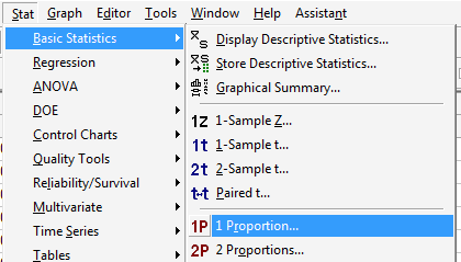
Under the Stat menu, select Basic Statistics, and then 1 Proportion...:
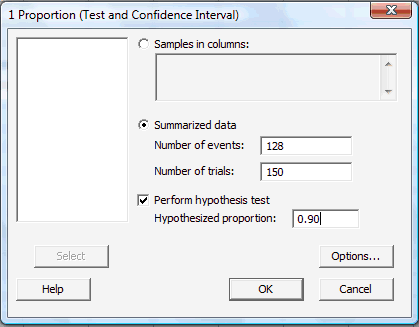
In the pop-up window that appears, click on the radio button labeled Summarized data. In the box labeled Number of events, type in the number of successes or events of interest, and in the box labeled Number of trials, type in the sample size n. Click on the box labeled Perform hypothesis test, and in the box labeled Hypothesized proportion, type in the value of the proportion assumed in the null hypothesis:
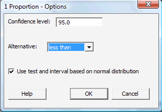
Click on the button labeled Options... In the pop-up window that appears, for the box labeled Alternative, select either less than, greater than, or not equal depending on the direction of the alternative hypothesis. Click on the box labeled Use test and interval based on normal distribution:

Then, click OK to return to the main pop-up window.

Then, upon clicking OK on the main pop-up window, the output should appear in the Session window:

Test of P = 0.9 vs p < 0.9
Sample	X	N	Sample P	95% Upper Bound	Z-Value	P-Value
1	128	150	0.853333	0.900846	-1.91	0.028

Using the normal approximation.

As you can see, Minitab reports not only the value of the test statistic (Z = −1.91) but also the P-value (0.028) and the 95% confidence interval (one-sided in this case, because of the one-sided hypothesis).

Hypothesis Test for Comparing Two Proportions

To illustrate how to tell Minitab to perform a Z-test for comparing two population proportions, let's refer to the smoker survey example that appeared on the page called Comparing Two Proportions.

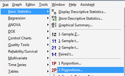
Under the Stat menu, select Basic Statistics, and then 2 Proportions...:
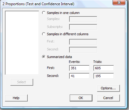
In the pop-up window that appears, click on the radio button labeled Summarized data. In the boxes labeled Events, type in the number of successes or events of interest for both the First and Second samples. And in the boxes labeled Trials, type in the size $n_{1}$ of the First sample and the size $n_{2}$ of the Second sample:
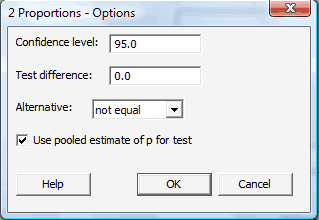
Click on the button labeled Options... In the pop-up window that appears, in the box labeled Test difference, type in the assumed value of the difference in the proportions that appears in the null hypothesis. The default value is 0.0, the value most commonly assumed, as it means that we are interested in testing for the equality of the population proportions. For the box labeled Alternative, select either less than, greater than, or not equal depending on the direction of the alternative hypothesis. Click on the box labeled Use pooled estimate of p for test:

Then, click OK to return to the main pop-up window.
Then, upon clicking OK on the main pop-up window, the output should appear in the Session window:

Sample X N Sample P

1 351 605 0.580165

2 41 195 0.210256

Difference = p (1) - p (2)
Estimate for difference: 0.369909
95% CI for difference: (0.0300499, 0.439319)
T-Test of difference = 0 (vs not =0): Z = 8.99 P-Value = 0.000

Fischer's exact test: P-Value = 0.000

Again, as you can see, Minitab reports not only the value of the test statistic (Z = 8.99) but other useful things as well, including the P-value, which in this case is so small as to be deemed to be 0.000 to three digits. For scientific reporting purposes, we would typically write that as P < 0.0001.

Sample	X	N	Sample P
1	351	605	0.580165
2	41	195	0.210256

Lesson 10: Tests About One Mean

Overview

In this lesson, we'll continue our investigation of hypothesis testing. In this case, we'll focus our attention on a hypothesis test for a population mean $μ$ for three situations:

a hypothesis test based on the normal distribution for the mean $μ$ for the completely unrealistic situation that the population variance $σ^{2}$ is known
a hypothesis test based on the $t$ -distribution for the mean $μ$ for the (much more) realistic situation that the population variance $σ^{2}$ is unknown
a hypothesis test based on the $t$ -distribution for $μ_{D}$ , the mean difference in the responses of two dependent populations

10.1 - Z-Test: When Population Variance is Known

Let's start by acknowledging that it is completely unrealistic to think that we'd find ourselves in the situation of knowing the population variance, but not the population mean. Therefore, the hypothesis testing method that we learn on this page has limited practical use. We study it only because we'll use it later to learn about the "power" of a hypothesis test (by learning how to calculate Type II error rates). As usual, let's start with an example.

Example 10-1

Boys of a certain age are known to have a mean weight of $μ = 85$ pounds. A complaint is made that the boys living in a municipal children's home are underfed. As one bit of evidence, $n = 25$ boys (of the same age) are weighed and found to have a mean weight of $\bar{x}$ = 80.94 pounds. It is known that the population standard deviation $σ$ is 11.6 pounds (the unrealistic part of this example!). Based on the available data, what should be concluded concerning the complaint?

Answer

The null hypothesis is $H_{0} : μ = 85$ , and the alternative hypothesis is $H_{A} : μ < 85$ . In general, we know that if the weights are normally distributed, then:

$Z = \frac{\bar{X} - μ}{σ / \sqrt{n}}$

follows the standard normal $N (0, 1)$ distribution. It is actually a bit irrelevant here whether or not the weights are normally distributed, because the same size $n = 25$ is large enough for the Central Limit Theorem to apply. In that case, we know that $Z$ , as defined above, follows at least approximately the standard normal distribution. At any rate, it seems reasonable to use the test statistic:

$Z = \frac{\bar{X} - μ_{0}}{σ / \sqrt{n}}$

for testing the null hypothesis

$H_{0} : μ = μ_{0}$

against any of the possible alternative hypotheses $H_{A} : μ \neq μ_{0}$ , $H_{A} : μ < μ_{0}$ , and $H_{A} : μ > μ_{0}$ .

For the example in hand, the value of the test statistic is:

$Z = \frac{80.94 - 85}{11.6 / \sqrt{25}} = - 1.75$

The critical region approach tells us to reject the null hypothesis at the $α = 0.05$ level if $Z < - 1.645$ . Therefore, we reject the null hypothesis because $Z = - 1.75 < - 1.645$ , and therefore falls in the rejection region:

As always, we draw the same conclusion by using the $p$ -value approach. Recall that the $p$ -value approach tells us to reject the null hypothesis at the $α = 0.05$ level if the $p$ -value $\leq α = 0.05$ . In this case, the $p$ -value is $P (Z < - 1.75) = 0.0401$ :

As expected, we reject the null hypothesis because the $p$ -value $= 0.0401 < α = 0.05$ .

By the way, we'll learn how to ask Minitab to conduct the $Z$ -test for a mean $μ$ in a bit, but this is what the Minitab output for this example looks like this:

Test of mu = 85 vs < 85
The assumed standard deviation = 11.6
N	Mean	SE Mean	95% Upper Bound	Z	P
25	80.9400	2.3200	84.7561	-1.75	0.040

10.2 - T-Test: When Population Variance is Unknown

Now that, for purely pedagogical reasons, we have the unrealistic situation (of a known population variance) behind us, let's turn our attention to the realistic situation in which both the population mean and population variance are unknown.

Example 10-2

It is assumed that the mean systolic blood pressure is $μ$ = 120 mm Hg. In the Honolulu Heart Study, a sample of $n = 100$ people had an average systolic blood pressure of 130.1 mm Hg with a standard deviation of 21.21 mm Hg. Is the group significantly different (with respect to systolic blood pressure!) from the regular population?

Answer

The null hypothesis is $H_{0} : μ = 120$ , and because there is no specific direction implied, the alternative hypothesis is $H_{A} : μ \neq 120$ . In general, we know that if the data are normally distributed, then:

$T = \frac{\bar{X} - μ}{S / \sqrt{n}}$

follows a $t$ -distribution with $n - 1$ degrees of freedom. Therefore, it seems reasonable to use the test statistic:

$T = \frac{\bar{X} - μ_{0}}{S / \sqrt{n}}$

for testing the null hypothesis $H_{0} : μ = μ_{0}$ against any of the possible alternative hypotheses $H_{A} : μ \neq μ_{0}$ , $H_{A} : μ < μ_{0}$ , and $H_{A} : μ > μ_{0}$ . For the example in hand, the value of the test statistic is:

$t = \frac{130.1 - 120}{21.21 / \sqrt{100}} = 4.762$

The critical region approach tells us to reject the null hypothesis at the $α = 0.05$ level if $t \geq t_{0.025, 99} = 1.9842$ or if $t \leq t_{0.025, 99} = - 1.9842$ . Therefore, we reject the null hypothesis because $t = 4.762 > 1.9842$ , and therefore falls in the rejection region:

Again, as always, we draw the same conclusion by using the $p$ -value approach. The $p$ -value approach tells us to reject the null hypothesis at the $α = 0.05$ level if the $p$ -value $\leq α = 0.05$ . In this case, the $p$ -value is $2 \times P (T_{99} > 4.762) < 2 \times P (T_{99} > 1.9842) = 2 (0.025) = 0.05$ :

As expected, we reject the null hypothesis because $p$ -value $\leq 0.01 < α = 0.05$ .

Again, we'll learn how to ask Minitab to conduct the t-test for a mean $μ$ in a bit, but this is what the Minitab output for this example looks like:

Test of mu = 120 vs not = 120
N	Mean	StDev	SE Mean	95% CI	T	P
100	130.100	21.210	2.121	(125.891, 134.309)	4.76	0.000

By the way, the decision to reject the null hypothesis is consistent with the one you would make using a 95% confidence interval. Using the data, a 95% confidence interval for the mean $μ$ is:

$\bar{x} \pm t_{0.025, 99} (\frac{s}{\sqrt{n}}) = 130.1 \pm 1.9842 (\frac{21.21}{\sqrt{100}})$

which simplifies to $130.1 \pm 4.21$ . That is, we can be 95% confident that the mean systolic blood pressure of the Honolulu population is between 125.89 and 134.31 mm Hg. How can a population living in a climate with consistently sunny 80 degree days have elevated blood pressure?!

Anyway, the critical region approach for the $α = 0.05$ hypothesis test tells us to reject the null hypothesis that $μ = 120$ :

if $t = \frac{\bar{x} - μ_{0}}{s / \sqrt{n}} \geq 1.9842$ or if $t = \frac{\bar{x} - μ_{0}}{s / \sqrt{n}} \leq - 1.9842$

which is equivalent to rejecting:

if $\bar{x} - μ_{0} \geq 1.9842 (\frac{s}{\sqrt{n}})$ or if $\bar{x} - μ_{0} \leq - 1.9842 (\frac{s}{\sqrt{n}})$

which is equivalent to rejecting:

if $μ_{0} \leq \bar{x} - 1.9842 (\frac{s}{\sqrt{n}})$ or if $μ_{0} \geq \bar{x} + 1.9842 (\frac{s}{\sqrt{n}})$

which, upon inserting the data for this particular example, is equivalent to rejecting:

if $μ_{0} \leq 125.89$ or if $μ_{0} \geq 134.31$

which just happen to be (!) the endpoints of the 95% confidence interval for the mean. Indeed, the results are consistent!

10.3 - Paired T-Test

In the next lesson, we'll learn how to compare the means of two independent populations, but there may be occasions in which we are interested in comparing the means of two dependent populations. For example, suppose a researcher is interested in determining whether the mean IQ of the population of first-born twins differs from the mean IQ of the population of second-born twins. She identifies a random sample of $n$ pairs of twins, and measures $X$ , the IQ of the first-born twin, and $Y$ , the IQ of the second-born twin. In that case, she's interested in determining whether:

$μ_{X} = μ_{Y}$

or equivalently if:

$μ_{X} - μ_{Y} = 0$

Now, the population of first-born twins is not independent of the population of second-born twins. Since all of our distributional theory requires the independence of measurements, we're rather stuck. There's a way out though... we can "remove" the dependence between $X$ and $Y$ by subtracting the two measurements $X_{i}$ and $Y_{i}$ for each pair of twins $i$ , that is, by considering the independent measurements

$D_{i} = X_{i} - Y_{i}$

Then, our null hypothesis involves just a single mean, which we'll denote $μ_{D}$ , the mean of the differences:

$H_{0} = μ_{D} = μ_{X} - μ_{Y} = 0$

and then our hard work is done! We can just use the $t$ -test for a mean for conducting the hypothesis test... it's just that, in this situation, our measurements are differences $d_{i}$ whose mean is $\bar{d}$ and standard deviation is $s_{D}$ . That is, when testing the null hypothesis $H_{0} : μ_{D} = μ_{0}$ against any of the alternative hypotheses $H_{A} : μ_{D} \neq μ_{0}$ , $H_{A} : μ_{D} < μ_{0}$ , and $H_{A} : μ_{D} > μ_{0}$ , we compare the test statistic:

$t = \frac{\bar{d} - μ_{0}}{s_{D} / \sqrt{n}}$

to a $t$ -distribution with $n - 1$ degrees of freedom. Let's take a look at an example!

Example 10-3

Blood samples from $n = 10$ = 10 people were sent to each of two laboratories (Lab 1 and Lab 2) for cholesterol determinations. The resulting data are summarized here:

Subject	Lab 1	Lab 2	Diff
1	296	318	-22
2	268	287	-19
.	.	.	.
.	.	.	.
.	.	.	.
10	262	285	-23
	${\bar{x}}_{1} = 260.6$	${\bar{x}}_{2} = 275$	$\begin{matrix} \bar{d} = - 14.4 \\ s_{d} = 6.77 \end{matrix}$

Is there a statistically significant difference at the $α = 0.01$ level, say, in the (population) mean cholesterol levels reported by Lab 1 and Lab 2?

Answer

The null hypothesis is $H_{0} : μ_{D} = 0$ , and the alternative hypothesis is $H_{A} : μ_{D} \neq 0$ . The value of the test statistic is:

$t = \frac{- 14.4 - 0}{6.77 / \sqrt{10}} = - 6.73$

The critical region approach tells us to reject the null hypothesis at the $α = 0.01$ level if $t > t_{0.005, 9} = 3.25$ or if $t < t_{0.005, 9} = - 3.25$ . Therefore, we reject the null hypothesis because $t = - 6.73 < - 3.25$ , and therefore falls in the rejection region.

Again, we draw the same conclusion when using the $p$ -value approach. In this case, the $p$ -value is:

$p - value = 2 \times P (T_{9} < - 6.73) \leq 2 \times 0.005 = 0.01$

As expected, we reject the null hypothesis because $p$ -value $\leq 0.01 = α$ .

And, the Minitab output for this example looks like this:

Test of mu = 0 vs not = 0
N	Mean	StDev	SE Mean	95% CI	T	P
10	-14.4000	6.7700	2.1409	(-19.2430, -9.5570)	-6.73	0.000

10.4 - Using Minitab

Z-Test for a Single Mean

To illustrate how to tell Minitab to perform a Z-test for a single mean, let's refer to the boys weight example that appeared on the page called The Z-test: When Population Variance is Known.

Under the Stat menu, select Basic Statistics, and then 1-Sample Z...:
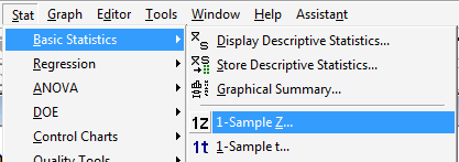
In the pop-up window that appears, click on the radio button labeled Summarized data. In the box labeled Sample size, type in the sample size n, and in the box labeled Mean, type in the sample mean. In the box labeled Standard deviation, type in the value of the known (or rather assumed!) population standard deviation. Click on the box labeled Perform hypothesis test, and in the box labeled Hypothesized mean, type in the value of the mean assumed in the null hypothesis:
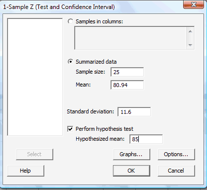
Click on the button labeled Options... In the pop-up window that appears, for the box labeled Alternative, select either less than, greater than, or not equal depending on the direction of the alternative hypothesis:

Then, click OK to return to the main pop-up window.

Then, upon clicking OK on the main pop-up window, the output should appear in the Session window:

Test of mu = 85 vs < 85
The assumed standard deviation = 11.6
N	Mean	SE Mean	95% Upper Bound	Z	P
25	80.94	2.32	84.76	-1.75	0.040

T-test for a Single Mean

To illustrate how to tell Minitab to perform a t-test for a single mean, let's refer to the systolic blood pressure example that appeared on the page called The T-test: When Population Variance is Unknown.

Under the Stat menu, select Basic Statistics, and then 1-Sample t...:
In the pop-up window that appears, click on the radio button labeled Summarized data. In the box labeled Sample size, type in the sample size n; in the box labeled Mean, type in the sample mean; and in the box labeled Standard deviation, type in the sample standard deviation. Click on the box labeled Perform hypothesis test, and in the box labeled Hypothesized mean, type in the value of the mean assumed in the null hypothesis:
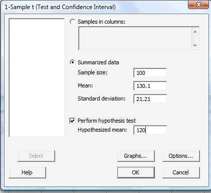
Click on the button labeled Options... In the pop-up window that appears, for the box labeled Alternative, select either less than, greater than, or not equal depending on the direction of the alternative hypothesis:

Then, click OK to return to the main pop-up window.

Then, upon clicking OK on the main pop-up window, the output should appear in the Session window:

Test of mu = 120 vs not = 120
N	Mean	StDev	SE Mean	95% CI	T	P
100	130.10	21.21	2.12	(125.89, 134.31)	4.76	0.000

(5) Note that a paired t-test can be performed in the same way. The summarized sample data would simply be the summarized differences. The extra step of calculating the differences would be required, however, if your data are the raw measurements from the two dependent samples. That is, if you have two columns containing, say, Before and After measurements for which you want to analyze Diff, their differences, you can use Minitab's calculator (under the Calc menu, select Calculator) to calculate the differences:

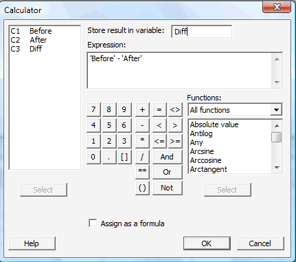
Upon clicking OK, the differences (Diff) should appear in your worksheet:

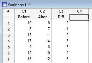
When performing the t-test, you'll then need to tell Minitab (in the Samples in columns box) that the differences are contained in the Diff column:

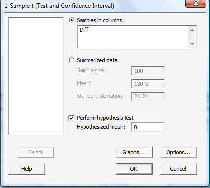
Here's what the paired t-test output would look like for this example:

One Sample T: Diff
Test of mu = 0 vs not = 0

Variable N Mean StDev SE Mean 95% CI T P

Diff 7 2.000 1.414 0.535 (0.692, 3.308) 3.74 0.010

Variable	N	Mean	StDev	SE Mean	95% CI	T	P
Diff	7	2.000	1.414	0.535	(0.692, 3.308)	3.74	0.010

Lesson 11: Tests of the Equality of Two Means

Overview

In this lesson, we'll continue our investigation of hypothesis testing. In this case, we'll focus our attention on a hypothesis test for the difference in two population means $μ_{1} - μ_{2}$ for two situations:

a hypothesis test based on the $t$ -distribution, known as the pooled two-sample $t$ -test, for $μ_{1} - μ_{2}$ when the (unknown) population variances $σ_{X}^{2}$ and $σ_{Y}^{2}$ are equal
a hypothesis test based on the $t$ -distribution, known as Welch's $t$ -test, for $μ_{1} - μ_{2}$ when the (unknown) population variances $σ_{X}^{2}$ and $σ_{Y}^{2}$ are not equal

Of course, because population variances are generally not known, there is no way of being 100% sure that the population variances are equal or not equal. In order to be able to determine, therefore, which of the two hypothesis tests we should use, we'll need to make some assumptions about the equality of the variances based on our previous knowledge of the populations we're studying.

11.1 - When Population Variances Are Equal

Let's start with the good news, namely that we've already done the dirty theoretical work in developing a hypothesis test for the difference in two population means $μ_{1} - μ_{2}$ when we developed a $(1 - α) 100 %$ confidence interval for the difference in two population means. Recall that if you have two independent samples from two normal distributions with equal variances $σ_{X}^{2} = σ_{Y}^{2} = σ^{2}$ , then:

$T = \frac{(\bar{X} - \bar{Y}) - (μ_{X} - μ_{Y})}{S_{p} \sqrt{\frac{1}{n} + \frac{1}{m}}}$

follows a $t_{n + m - 2}$ distribution where $S_{p}^{2}$ , the pooled sample variance:

$S_{p}^{2} = \frac{(n - 1) S_{X}^{2} + (m - 1) S_{Y}^{2}}{n + m - 2}$

is an unbiased estimator of the common variance $σ^{2}$ . Therefore, if we're interested in testing the null hypothesis:

$H_{0} : μ_{X} - μ_{Y} = 0$ (or equivalently $H_{0} : μ_{X} = μ_{Y}$ )

against any of the alternative hypotheses:

$H_{A} : μ_{X} - μ_{Y} \neq 0, H_{A} : μ_{X} - μ_{Y} < 0, or H_{A} : μ_{X} - μ_{Y} > 0$

we can use the test statistic:

$T = \frac{(\bar{X} - \bar{Y}) - (μ_{X} - μ_{Y})}{S_{p} \sqrt{\frac{1}{n} + \frac{1}{m}}}$

and follow the standard hypothesis testing procedures. Let's take a look at an example.

Example 11-1

A psychologist was interested in exploring whether or not male and female college students have different driving behaviors. There were several ways that she could quantify driving behaviors. She opted to focus on the fastest speed ever driven by an individual. Therefore, the particular statistical question she framed was as follows:

Is the mean fastest speed driven by male college students different than the mean fastest speed driven by female college students?

She conducted a survey of a random $n = 34$ male college students and a random $m = 29$ female college students. Here is a descriptive summary of the results of her survey:

Males (X)	Females (Y)
$n = 34$ $\bar{x} = 105.5$ $s_{x} = 20.1$	$m = 29$ $\bar{y} = 90.9$ $s_{y} = 12.2$

and here is a graphical summary of the data in the form of a dotplot:

Is there sufficient evidence at the $α = 0.05$ level to conclude that the mean fastest speed driven by male college students differs from the mean fastest speed driven by female college students?

Answer

Because the observed standard deviations of the two samples are of similar magnitude, we'll assume that the population variances are equal. Let's also assume that the two populations of fastest speed driven for males and females are normally distributed. (We can confirm, or deny, such an assumption using a normal probability plot, but let's simplify our analysis for now.) The randomness of the two samples allows us to assume independence of the measurements as well.

Okay, assumptions all met, we can test the null hypothesis:

$H_{0} : μ_{M} - μ_{F} = 0$

against the alternative hypothesis:

$H_{A} : μ_{M} - μ_{F} \neq 0$

using the test statistic:

$t = \frac{(105.5 - 90.9) - 0}{16.9 \sqrt{\frac{1}{34} + \frac{1}{29}}} = 3.42$

because, among other things, the pooled sample standard deviation is:

$s_{p} = \sqrt{\frac{33 ({20.1}^{2}) + 28 ({12.2}^{2})}{61}} = 16.9$

The critical value approach tells us to reject the null hypothesis in favor of the alternative hypothesis if:

$| t | \geq t_{α / 2, n + m - 2} = t_{0.025, 61} = 1.9996$

We reject the null hypothesis because the test statistic ( $t = 3.42$ ) falls in the rejection region:

There is sufficient evidence at the $α = 0.05$ level to conclude that the average fastest speed driven by the population of male college students differs from the average fastest speed driven by the population of female college students.

Not surprisingly, the decision is the same using the $p$ -value approach. The $p$ -value is 0.0012:

$P = 2 \times P (T_{61} > 3.42) = 2 (0.0006) = 0.0012$

Therefore, because $p = 0.0012 \leq α = 0.05$ , we reject the null hypothesis in favor of the alternative hypothesis. Again, we conclude that there is sufficient evidence at the $α = 0.05$ level to conclude that the average fastest speed driven by the population of male college students differs from the average fastest speed driven by the population of female college students.

By the way, we'll see how to tell Minitab to conduct a two-sample t-test in a bit here, but in the meantime, this is what the output would look like:

Two-Sample T: For Fastest

Gender	N	Mean	StDev	SE Mean
1	34	105.5	20.1	3.4
2	29	90.9	12.2	2.3

Difference = mu (1) - mu (2)
Estimate for difference: 14.6085
95% CI for difference: (6.0630, 23.1540)
T-Test of difference = 0 (vs not =) : T-Value = 3.42 P-Value = 0.001 DF = 61
Both use Pooled StDev = 16.9066

11.2 - When Population Variances Are Not Equal

Let's again start with the good news that we've already done the dirty theoretical work here. Recall that if you have two independent samples from two normal distributions with unequal variances $σ_{X}^{2} \neq σ_{Y}^{2}$ , then:

$T = \frac{(\bar{X} - \bar{Y}) - (μ_{X} - μ_{Y})}{\sqrt{\frac{S_{X}^{2}}{n} + \frac{S_{Y}^{2}}{m}}}$

follows, at least approximately, a $t_{r}$ distribution where $r$ , the adjusted degrees of freedom is determined by the equation:

$r = \frac{{(\frac{s_{X}^{2}}{n} + \frac{s_{Y}^{2}}{m})}^{2}}{\frac{(s_{X}^{2} / n)^{2}}{n - 1} + \frac{(s_{Y}^{2} / m)^{2}}{m - 1}}$

If r doesn't equal an integer, as it usually doesn't, then we take the integer portion of $r$ . That is, we use $⌊ r ⌋$ if necessary.

With that now being recalled, if we're interested in testing the null hypothesis:

$H_{0} : μ_{X} - μ_{Y} = 0$ (or equivalently $H_{0} : μ_{X} = μ_{Y}$ )

against any of the alternative hypotheses:

$H_{A} : μ_{X} - μ_{Y} \neq 0, H_{A} : μ_{X} - μ_{Y} < 0, or H_{A} : μ_{X} - μ_{Y} > 0$

we can use the test statistic:

$T = \frac{(\bar{X} - \bar{Y}) - (μ_{X} - μ_{Y})}{\sqrt{\frac{S_{X}^{2}}{n} + \frac{S_{Y}^{2}}{m}}}$

and follow the standard hypothesis testing procedures. Let's return to our fastest speed driven example.

Example 11-1 (Continued)

A psychologist was interested in exploring whether or not male and female college students have different driving behaviors. There were a number of ways that she could quantify driving behaviors. She opted to focus on the fastest speed ever driven by an individual. Therefore, the particular statistical question she framed was as follows:

Is the mean fastest speed driven by male college students different than the mean fastest speed driven by female college students?

She conducted a survey of a random $n = 34$ male college students and a random $m = 29$ female college students. Here is a descriptive summary of the results of her survey:

Males (X)	Females (Y)
$n = 34$ $\bar{x} = 105.5$ $s_{x} = 20.1$	$m = 29$ $\bar{y} = 90.9$ $s_{y} = 12.2$

Is there sufficient evidence at the $α = 0.05$ level to conclude that the mean fastest speed driven by male college students differs from the mean fastest speed driven by female college students?

Answer

This time let's not assume that the population variances are equal. Then, we'll see if we arrive at a different conclusion. Let's still assume though that the two populations of fastest speed driven for males and females are normally distributed. And, we'll again permit the randomness of the two samples to allow us to assume independence of the measurements as well.

That said, then we can test the null hypothesis:

$H_{0} : μ_{M} - μ_{F} = 0$

against the alternative hypothesis:

$H_{A} : μ_{M} - μ_{F} \neq 0$

comparing the test statistic:

$t = \frac{(105.5 - 90.9) - 0}{\sqrt{\frac{{20.1}^{2}}{34} + \frac{{12.2}^{2}}{29}}} = 3.54$

to a $T$ distribution with $r$ degrees of freedom, where:

$r = \frac{{(\frac{{12.2}^{2}}{29} + \frac{{20.1}^{2}}{34})}^{2}}{(\frac{1}{28}) {(\frac{{12.2}^{2}}{29})}^{2} + (\frac{1}{33}) {(\frac{{20.1}^{2}}{34})}^{2}} = 55.5$

Oops... that's not an integer, so we're going to need to take the greatest integer portion of that $r$ . That is, we take the degrees of freedom to be $⌊ r ⌋ = ⌊ 55.5 ⌋ = 55$ .

Then, the critical value approach tells us to reject the null hypothesis in favor of the alternative hypothesis if:

$t > t_{0.025, 55} = 2.004$

We reject the null hypothesis because the test statistic ( $t = 3.54$ ) falls in the rejection region:

There is (again!) sufficient evidence at the $α = 0.05$ level to conclude that the average fastest speed driven by the population of male college students differs from the average fastest speed driven by the population of female college students.

And again, the decision is the same using the $p$ -value approach. The $p$ -value is 0.0008:

$P = 2 \times P (T_{55} > 3.54) = 2 (0.0004) = 0.0008$

Therefore, because $p = 0.008 \leq α = 0.05$ , we reject the null hypothesis in favor of the alternative hypothesis. Again, we conclude that there is sufficient evidence at the $α = 0.05$ level to conclude that the average fastest speed driven by the population of male college students differs from the average fastest speed driven by the population of female college students.

At any rate, we see that in this case, our conclusion is the same regardless of whether or not we assume equality of the population variances.

And, just in case you're interested... we'll see how to tell Minitab to conduct a Welch's $t$ -test very soon, but in the meantime, this is what the output would look like for this example:

Two-Sample T: For Fastest

Gender	N	Mean	StDev	SE Mean
1	34	105.5	20.1	3.4
2	29	90.9	12.2	2.3

Difference = mu (1) - mu (2)
Estimate for difference: 14.6085
95% CI for difference: (6.3575, 22.8596)
T-Test of difference = 0 (vs not =) : T-Value = 3.55 P-Value = 0.001 DF = 55

11.3 - Using Minitab

Just as is the case for asking Minitab to calculate pooled t-intervals and Welch's t-intervals for $μ_{1} - μ_{2}$ , the commands necessary for asking Minitab to perform a two-sample t-test or a Welch's t-test depend on whether the data are entered in two columns, or the data are entered in one column with a grouping variable in a second column.

Let's recall the spider and prey example, in which the feeding habits of two species of net-casting spiders were studied. The species, the deinopis, and menneus coexist in eastern Australia. The following data were obtained on the size, in millimeters, of the prey of random samples of the two species:

Size of Random Pray Samples of the Deinopis Spider in Millimeters
sample 1	sample 2	sample 3	sample 4	sample 5	sample 6	sample 7	sample 8	sample 9	sample 10
12.9	10.2	7.4	7.0	10.5	11.9	7.1	9.9	14.4	11.3

Size of Random Pray Samples of the Menneus Spider in Millimeters
sample 1	sample 2	sample 3	sample 4	sample 5	sample 6	sample 7	sample 8	sample 9	sample 10
10.2	6.9	10.9	11.0	10.1	5.3	7.5	10.3	9.2	8.8

Let's use the data and Minitab to test whether the mean prey size of the populations of the two types of spiders differs.

When the Data are Entered in Two Columns

Enter the data in two columns, such as:
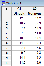
Under the Stat menu, select Basic Statistics, and then select 2-Sample t...:
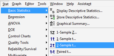
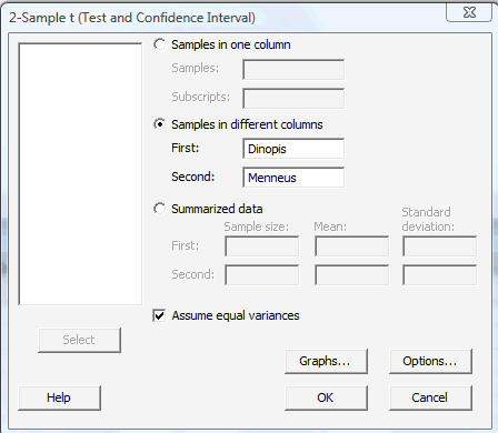
In the pop-up window that appears, select Samples in different columns. Specify the name of the First variable, and specify the name of the Second variable. For the two-sample (pooled) t-test, click on the box labeled Assume equal variances. (For Welch's t-test, leave the box labeled Assume equal variances unchecked.):
Click on the button labeled Options... In the pop-up window that appears, for the box labeled Alternative, select either less than, greater than, or not equal depending on the direction of the alternative hypothesis:

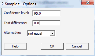
Then, click OK to return to the main pop-up window.

Then, upon clicking OK on the main pop-up window, the output should appear in the Session window:

Two-Sample T: For Deinopis vs Menneus
Variable	N	Mean	StDev	SE Mean
Deinopis	10	10.26	2.51	0.79
Menneus	10	9.02	1.90	0.60

Difference = mu (Deinopis) - mu (Menneus)
Estimate for difference: 1.240
95% CI for difference: (-0.852, 3.332)
T-Test of difference = 0 (vs not =): T-Value = 1.25 P-Value = 0.229 DF = 18
Both use Pooled StDev = 2.2266

When the Data are Entered in One Column, and a Grouping Variable in a Second Column

Enter the data in one column (called Prey, say), and the grouping variable in a second column (called Group, say, with 1 denoting a deinopis spider and 2 denoting a menneus spider), such as:
Under the Stat menu, select Basic Statistics, and then select 2-Sample t...:
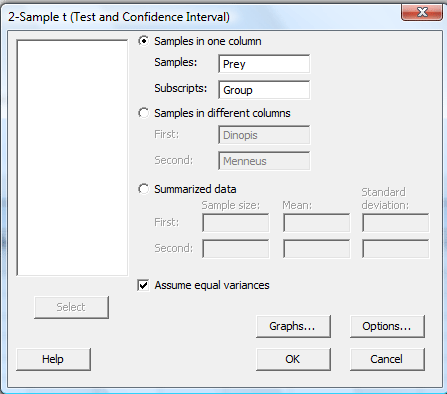
In the pop-up window that appears, select Samples in one column. Specify the name of the Samples variable (Prey, for us) and specify the name of the Subscripts (grouping) variable (Group, for us). For the two-sample (pooled) t-test, click on the box labeled Assume equal variances. (For Welch's t-test, leave the box labeled Assume equal variances unchecked.):
Click on the button labeled Options... In the pop-up window that appears, for the box labeled Alternative, select either less than, greater than, or not equal depending on the direction of the alternative hypothesis:

Then, click OK to return to the main pop-up window.
Then, upon clicking OK on the main pop-up window, the output should appear in the Session window:

Two-Sample T: For Prey

Group N Mean StDev SE Mean

1 10 10.26 2.51 0.79

2 10 9.02 1.90 0.60

Difference = mu (1) - mu (2)
Estimate for difference: 1.240
95% CI for difference: (-0.852, 3.332)
T-Test of difference = 0 (vs not =): T-Value = 1.25 P-Value = 0.229 DF = 18
Both use Pooled StDev = 2.2266

Group	N	Mean	StDev	SE Mean
1	10	10.26	2.51	0.79
2	10	9.02	1.90	0.60

Lesson 12: Tests for Variances

Continuing our development of hypothesis tests for various population parameters, in this lesson, we'll focus on hypothesis tests for population variances. Specifically, we'll develop:

a hypothesis test for testing whether a single population variance $σ^{2}$ equals a particular value
a hypothesis test for testing whether two population variances are equal

12.1 - One Variance

Yeehah again! The theoretical work for developing a hypothesis test for a population variance $σ^{2}$ is already behind us. Recall that if you have a random sample of size n from a normal population with (unknown) mean $μ$ and variance $σ^{2}$ , then:

$χ^{2} = \frac{(n - 1) S^{2}}{σ^{2}}$

follows a chi-square distribution with n−1 degrees of freedom. Therefore, if we're interested in testing the null hypothesis:

$H_{0} : σ^{2} = σ_{0}^{2}$

against any of the alternative hypotheses:

$H_{A} : σ^{2} \neq σ_{0}^{2}, H_{A} : σ^{2} < σ_{0}^{2}, or H_{A} : σ^{2} > σ_{0}^{2}$

we can use the test statistic:

$χ^{2} = \frac{(n - 1) S^{2}}{σ_{0}^{2}}$

and follow the standard hypothesis testing procedures. Let's take a look at an example.

Example 12-1

A manufacturer of hard safety hats for construction workers is concerned about the mean and the variation of the forces its helmets transmits to wearers when subjected to an external force. The manufacturer has designed the helmets so that the mean force transmitted by the helmets to the workers is 800 pounds (or less) with a standard deviation to be less than 40 pounds. Tests were run on a random sample of n = 40 helmets, and the sample mean and sample standard deviation were found to be 825 pounds and 48.5 pounds, respectively.

Do the data provide sufficient evidence, at the $α = 0.05$ level, to conclude that the population standard deviation exceeds 40 pounds?

Answer

We're interested in testing the null hypothesis:

$H_{0} : σ^{2} = 40^{2} = 1600$

against the alternative hypothesis:

$H_{A} : σ^{2} > 1600$

Therefore, the value of the test statistic is:

$χ^{2} = \frac{(40 - 1) {48.5}^{2}}{40^{2}} = 57.336$

Is the test statistic too large for the null hypothesis to be true? Well, the critical value approach would have us finding the threshold value such that the probability of rejecting the null hypothesis if it were true, that is, of committing a Type I error, is small... 0.05, in this case. Using Minitab (or a chi-square probability table), we see that the cutoff value is 54.572:

That is, we reject the null hypothesis in favor of the alternative hypothesis if the test statistic $χ^{2}$ is greater than 54.572. It is. That is, the test statistic falls in the rejection region:

Therefore, we conclude that there is sufficient evidence, at the 0.05 level, to conclude that the population standard deviation exceeds 40.

Of course, the P-value approach yields the same conclusion. In this case, the P-value is the probablity that we would observe a chi-square(39) random variable more extreme than 57.336:

As the drawing illustrates, the P-value is 0.029 (as determined using the chi-square probability calculator in Minitab). Because $P = 0.029 \leq 0.05$ , we reject the null hypothesis in favor of the alternative hypothesis.

Do the data provide sufficient evidence, at the $α = 0.05$ level, to conclude that the population standard deviation differs from 40 pounds?

Answer

In this case, we're interested in testing the null hypothesis:

$H_{0} : σ^{2} = 40^{2} = 1600$

against the alternative hypothesis:

$H_{A} : σ^{2} \neq 1600$

The value of the test statistic remains the same. It is again:

$χ^{2} = \frac{(40 - 1) {48.5}^{2}}{40^{2}} = 57.336$

Now, is the test statistic either too large or too small for the null hypothesis to be true? Well, the critical value approach would have us dividing the significance level $α = 0.05$ into 2, to get 0.025, and putting one of the halves in the left tail, and the other half in the other tail. Doing so (and using Minitab to get the cutoff values), we get that the lower cutoff value is 23.654 and the upper cutoff value is 58.120:

That is, we reject the null hypothesis in favor of the two-sided alternative hypothesis if the test statistic $χ^{2}$ is either smaller than 23.654 or greater than 58.120. It is not. That is, the test statistic does not fall in the rejection region:

Therefore, we fail to reject the null hypothesis. There is insufficient evidence, at the 0.05 level, to conclude that the population standard deviation differs from 40.

Of course, the P-value approach again yields the same conclusion. In this case, we simply double the P-value we obtained for the one-tailed test yielding a P-value of 0.058:

$P = 2 \times P (χ_{39}^{2} > 57.336) = 2 \times 0.029 = 0.058$

Because $P = 0.058 > 0.05$ , we fail to reject the null hypothesis in favor of the two-sided alternative hypothesis.

The above example illustrates an important fact, namely, that the conclusion for the one-sided test does not always agree with the conclusion for the two-sided test. If you have reason to believe that the parameter will differ from the null value in a particular direction, then you should conduct the one-sided test.

12.2 - Two Variances

Let's now recall the theory necessary for developing a hypothesis test for testing the equality of two population variances. Suppose $X_{1}, X_{2}, \dots, X_{n}$ is a random sample of size n from a normal population with mean $μ_{X}$ and variance $σ_{X}^{2}$ . And, suppose, independent of the first sample, $Y_{1}, Y_{2}, \dots, Y_{m}$ is another random sample of size m from a normal population with $μ_{Y}$ and variance $σ_{Y}^{2}$ . Recall then, in this situation, that:

$\frac{(n - 1) S_{X}^{2}}{σ_{X}^{2}} and \frac{(m - 1) S_{Y}^{2}}{σ_{Y}^{2}}$

have independent chi-square distributions with n−1 and m−1 degrees of freedom, respectively. Therefore:

$F = \frac{[\frac{(n - 1) S_{X}^{2}}{σ_{x}^{2}} / (n - 1)]}{[\frac{(m - 1) S_{Y}^{2}}{σ_{Y}^{2}} / (m - 1)]} = \frac{S_{X}^{2}}{S_{Y}^{2}} \cdot \frac{σ_{Y}^{2}}{σ_{X}^{2}}$

follows an F distribution with n−1 numerator degrees of freedom and m−1 denominator degrees of freedom. Therefore, if we're interested in testing the null hypothesis:

$H_{0} : σ_{X}^{2} = σ_{Y}^{2}$ (or equivalently $H_{0} : \frac{σ_{Y}^{2}}{σ_{X}^{2}} = 1$ )

against any of the alternative hypotheses:

$H_{A} : σ_{X}^{2} \neq σ_{Y}^{2}, H_{A} : σ_{X}^{2} > σ_{Y}^{2}, or H_{A} : σ_{X}^{2} < σ_{Y}^{2}$

we can use the test statistic:

$F = \frac{S_{X}^{2}}{S_{Y}^{2}}$

and follow the standard hypothesis testing procedures. When doing so, we might also want to recall this important fact about the F-distribution:

$F_{1 - (α / 2)} (n - 1, m - 1) = \frac{1}{F_{α / 2} (m - 1, n - 1)}$

so that when we use the critical value approach for a two-sided alternative:

$H_{A} : σ_{X}^{2} \neq σ_{Y}^{2}$

we reject if the test statistic F is too large:

$F \geq F_{α / 2} (n - 1, m - 1)$

or if the test statistic F is too small:

$F \leq F_{1 - (α / 2)} (n - 1, m - 1) = \frac{1}{F_{α / 2} (m - 1, n - 1)}$

Okay, let's take a look at an example. In the last lesson, we performed a two-sample t-test (as well as Welch's test) to test whether the mean fastest speed driven by the population of male college students differs from the mean fastest speed driven by the population of female college students. When we performed the two-sample t-test, we just assumed the population variances were equal. Let's revisit that example again to see if our assumption of equal variances is valid.

Example 12-2

A psychologist was interested in exploring whether or not male and female college students have different driving behaviors. The particular statistical question she framed was as follows:

Is the mean fastest speed driven by male college students different than the mean fastest speed driven by female college students?

The psychologist conducted a survey of a random $n = 34$ male college students and a random $m = 29$ female college students. Here is a descriptive summary of the results of her survey:

Males (X)	Females (Y)
$n = 34$ $\bar{x} = 105.5$ $s_{x} = 20.1$	$m = 29$ $\bar{y} = 90.9$ $s_{y} = 12.2$

Is there sufficient evidence at the $α = 0.05$ level to conclude that the variance of the fastest speed driven by male college students differs from the variance of the fastest speed driven by female college students?

Answer

We're interested in testing the null hypothesis:

$H_{0} : σ_{X}^{2} = σ_{Y}^{2}$

against the alternative hypothesis:

$H_{A} : σ_{X}^{2} \neq σ_{Y}^{2}$

The value of the test statistic is:

$F = \frac{{12.2}^{2}}{{20.1}^{2}} = 0.368$

(Note that I intentionally put the variance of what we're calling the Y sample in the numerator and the variance of what we're calling the X sample in the denominator. I did this only so that my results match the Minitab output we'll obtain on the next page. In doing so, we just need to make sure that we keep track of the correct numerator and denominator degrees of freedom.) Using the critical value approach, we divide the significance level $α = 0.05$ into 2, to get 0.025, and put one of the halves in the left tail, and the other half in the other tail. Doing so, we get that the lower cutoff value is 0.478 and the upper cutoff value is 2.0441:

Because the test statistic falls in the rejection region, that is, because $F = 0.368 \leq 0.478$ , we reject the null hypothesis in favor of the alternative hypothesis. There is sufficient evidence at the $α = 0.05$ level to conclude that the population variances are not equal. Therefore, the assumption of equal variances that we made when performing the two-sample t-test on these data in the previous lesson does not appear to be valid. It would behoove us to use Welch's t-test instead.

12.3 - Using Minitab

In each case, we'll illustrate how to perform the hypothesis tests of this lesson using summarized data.

Hypothesis Test for One Variance

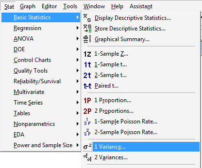
Under the Stat menu, select Basic Statistics, and then select 1 Variance...:
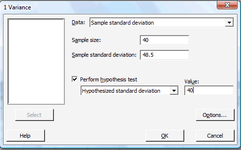
In the pop-up window that appears, in the box labeled Data, select Sample standard deviation (or alternatively Sample variance). In the box labeled Sample size, type in the size n of the sample. In the box labeled Sample standard deviation, type in the sample standard deviation. Click on the box labeled Perform hypothesis test, and in the box labeled Value, type in the Hypothesized standard deviation (or alternatively the Hypothesized variance):
Click on the button labeled Options... In the pop-up window that appears, for the box labeled Alternative, select either less than, greater than, or not equal depending on the direction of the alternative hypothesis:

Then, click on OK to return to the main pop-up window.
Then, upon clicking OK on the main pop-up window, the output should appear in the Session window:

95% Confidence Intervals

Method CI for
StDev CI for
Variance

Chi-Square (39.7, 62.3) (1578, 3878)

Tests

Method Test
Statistic DF P-Value

Chi-Square 57.34 39 0.059

Method	CI for StDev	CI for Variance
Chi-Square	(39.7, 62.3)	(1578, 3878)

Method	Test Statistic	DF	P-Value
Chi-Square	57.34	39	0.059

Hypothesis Test for Two Variances

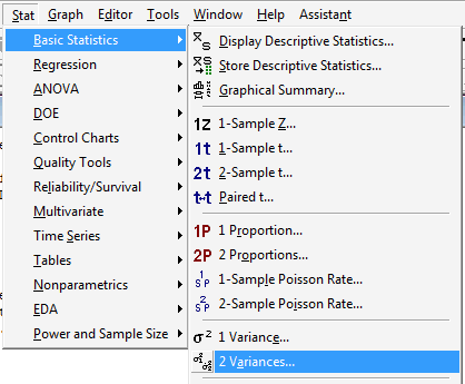
Under the Stat menu, select Basic Statistics, and then select 2 Variances...:
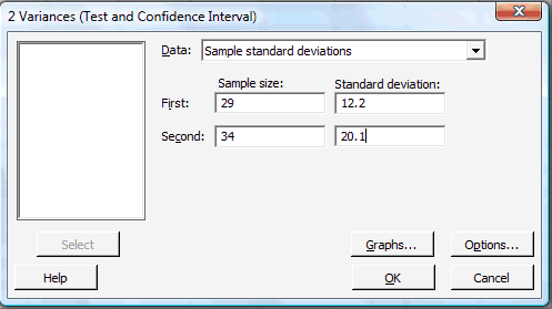
In the pop-up window that appears, in the box labeled Data, select Sample standard deviations (or alternatively Sample variances). In the box labeled Sample size, type in the size n of the First sample and m of the Second sample. In the box labeled Standard deviation, type in the sample standard deviations for the First and Second samples:
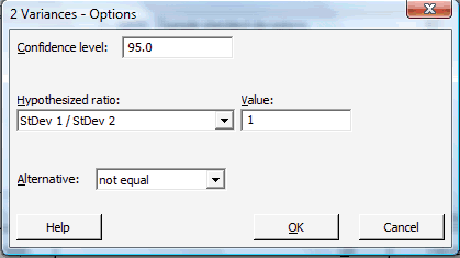
Click on the button labeled Options... In the pop-up window that appears, in the box labeled Value, type in the Hypothesized ratio of the standard deviations (or the Hypothesized ratio of the variances). For the box labeled Alternative, select either less than, greater than, or not equal depending on the direction of the alternative hypothesis:

Then, click on OK to return to the main pop-up window.
1. Then, upon clicking OK on the main pop-up window, the output should appear in the Session window:
  
  Test and CI for Two Variances
  
  Method
  
  Null hypothesis                 Sigma(1) / Sigma(2) = 1
  Alternative hypothesis     Sigma(1) / Sigma(2) not = 1
  Significance level              Alpha = 0.05
  
  Statistics
  
  Sample N StDev Variance
  
  1 29 12.200 148.840
  
  2 34 20.100 404.010
  
  Ratio of standard deviations = 0.607
  Ratio of variances = 0.368
  
  95% Confidence Intervals
  
  Distribution
  of Data CI for StDev Ratio CI for
  Variance Ratio
  
  Normal (0.425, 0.877) (0.180, 0.770)
  
  Tests
  
  Method DF1 DF2 Test
  Statistic P-Value
  
  F Test (normal) 28 33 0.37 0.009

Sample	N	StDev	Variance
1	29	12.200	148.840
2	34	20.100	404.010

Distribution of Data	CI for StDev Ratio	CI for Variance Ratio
Normal	(0.425, 0.877)	(0.180, 0.770)

Method	DF1	DF2	Test Statistic	P-Value
F Test (normal)	28	33	0.37	0.009

Lesson 13: One-Factor Analysis of Variance

We previously learned how to compare two population means using either the pooled two-sample t-test or Welch's t-test. What happens if we want to compare more than two means? In this lesson, we'll learn how to do just that. More specifically, we'll learn how to use the analysis of variance method to compare the equality of the (unknown) means $μ_{1}, μ_{2}, \dots, μ_{m}$ of m normal distributions with an unknown but common variance $σ^{2}$ . Take specific note about that last part.... "an unknown but common variance $σ^{2}$ ." That is, the analysis of variance method assumes that the population variances are equal. In that regard, the analysis of variance method can be thought of as an extension of the pooled two-sample t-test.

13.1 - The Basic Idea

We could take a top-down approach by first presenting the theory of analysis of variance and then following it up with an example. We're not going to do it that way though. We're going to take a bottom-up approach, in which we first develop the idea behind the analysis of variance on this page, and then present the results on the next page. Only after we've completed those two steps will we take a step back and look at the theory behind analysis of variance. That said, let's start with our first example of the lesson.

Example 13-1

A researcher for an automobile safety institute was interested in determining whether or not the distance that it takes to stop a car going 60 miles per hour depends on the brand of the tire. The researcher measured the stopping distance (in feet) of ten randomly selected cars for each of five different brands. So that he and his assistants would remain blinded, the researcher arbitrarily labeled the brands of the tires as Brand1, Brand2, Brand3, Brand4, and Brand5. Here are the data resulting from his experiment:

Brand1	Brand2	Brand3	Brand4	Brand5
194	189	185	183	195
184	204	183	193	197
189	190	186	184	194
189	190	183	186	202
188	189	179	194	200
186	207	191	199	211
195	203	188	196	203
186	193	196	188	206
183	181	189	193	202
188	206	194	196	195

Do the data provide enough evidence to conclude that at least one of the brands is different from the others with respect to stopping distance?

Answer

The first thing we might want to do is to create some sort of summary plot of the data. Here is a box plot of the data:

Hmmm. It appears that the box plots for Brand1 and Brand5 have very little, if any, overlap at all. The same can be said for Brand3 and Brand5. Here are some summary statistics of the data:

Brand	N	MEAN	SD
1	10	188.20	3.88
2	10	195.20	9.02
3	10	187.40	5.27
4	10	191.20	5.55
5	10	200.50	5.44

It appears that the sample means differ quite a bit. For example, the average stopping distance of Brand3 is 187.4 feet (with a standard deviation of 5.27 feet), while the average stopping distance of Brand5 is 200.5 feet (with a standard deviation of 5.44 feet). A difference of 13 feet could mean the difference between getting into an accident or not. But, of course, we can't draw conclusions about the performance of the brands based on one sample. After all, a different random sample of cars could yield different results. Instead, we need to use the sample means to try to draw conclusions about the population means.

More specifically, the researcher needs to test the null hypothesis that the group population means are all the same against the alternative that at least one group population mean differs from the others. That is, the researcher needs to test this null hypothesis:

$H_{0} : μ_{1} = μ_{2} = μ_{3} = μ_{4} = μ_{5}$

against this alternative hypothesis:

$H_{A} :$ at least one of the $μ_{i}$ differs from the others

In this lesson, we are going to learn how to use a method called analysis of variance to answer the researcher's question. Jumping right to the punch line, with no development or theoretical justification whatsoever, we'll use an analysis of variance table, such as this one:

Analysis of Variance for comparing all 5 brands
Source	DF	SS	MS	F	P
Brand	4	1174.8	293.7	7.95	0.000
Error	45	1661.7	36.9
Total	49	2836.5

to draw conclusions about the equality of two or more population means. And, as we always do when performing hypothesis tests, we'll compare the P-value to $α$ , our desired willingness to commit a Type I error. In this case, the researcher's P-value is very small (0.000, to three decimal places), so he should reject his null hypothesis. That is, there is sufficient evidence, at even a 0.01 level, to conclude that the mean stopping distance for at least one brand of tire is different than the mean stopping distances of the others.

So far, we have seen a typical null and alternative hypothesis in the analysis of variance framework, as well as an analysis of variance table. Let's take a look at another example with the idea of continuing to work on developing the basic idea behind the analysis of variance method.

Example 13-2

Suppose an education researcher is interested in determining whether a learning method affects students' exam scores. Specifically, suppose she considers these three methods:

standard
osmosis
shock therapy

Suppose she convinces 15 students to take part in her study, so she randomly assigns 5 students to each method. Then, after waiting eight weeks, she tests the students to get exam scores.

What would the researcher's data have to look like to be able to conclude that at least one of the methods yields different exam scores than the others?

Answer

Suppose a dot plot of the researcher's data looked like this:

What would we want to conclude? Well, there's a lot of separation in the data between the three methods. In this case, there is little variation in the data within each method, but a lot of variation in the data across the three methods. For these data, we would probably be willing to conclude that there is a difference between the three methods.

Now, suppose instead that a dot plot of the researcher's data looked like this:

What would we want to conclude? Well, there's less separation in the data between the three methods. In this case, there is a lot of variation in the data within each method, and still some variation in the data across the three methods, but not as much as in the previous dot plot. For these data, it is not as obvious that we can conclude that there is a difference between the three methods.

Let's consider one more possible dot plot:

What would we want to conclude here? Well, there's even less separation in the data between the three methods. In this case, there is a real lot of variation in the data within each method, and not much variation at all in the data across the three methods. For these data, we would probably want to conclude that there is no difference between the three methods.

If you go back and look at the three possible data sets, you'll see that we drew our conclusions by comparing the variation in the data within a method to the variation in the data across methods. Let's try to formalize that idea a bit more by revisiting the two most extreme examples. First, the example in which we concluded that the methods differ:

Let's quantify (or are we still just qualifying?) the amount of variation within a method by comparing the five data points within a method to the method's mean, as represented in the plot as a color-coded triangle. And, let's quantify (or qualify?) the amount of variation across the methods by comparing the method means, again represented in the plot as a color-coded triangle, to the overall grand mean, that is, the average of all fifteen data points (ignoring the method). In this case, the variation between the group means and the grand mean is larger than the variation within the groups.

Now, let's revisit the example in which we wanted to conclude that there was no difference in the three methods:

In this case, the variation between the group means and the grand mean is smaller than the variation within the groups.

Hmmm... these two examples suggest that our method should compare the variation between the groups to that of the variation within the groups. That's just what an analysis of variance does!

Let's see what conclusion we draw from an analysis of variance of these data. Here's the analysis of variance table for the first study, in which we wanted to conclude that there was a difference in the three methods:

Source	DF	SS	MS	F	P
Factor	2	2510.5	1255.3	93.44	0.000
Error	12	161.2	13.4
Total	14	2671.7

In this case, the P-value is small (0.000, to three decimal places). We can reject the null hypothesis of equal means at the 0.05 level. That is, there is sufficient evidence at the 0.05 level to conclude that the mean exam scores of the three study methods are significantly different.

Here's the analysis of variance table for the third study, in which we wanted to conclude that there was no difference in the three methods:

Source	DF	SS	MS	F	P
Factor	2	80.1	40.1	0.46	0.643
Error	12	1050.8	87.6
Total	14	1130.9

In this case, the P-value, 0.643, is large. We fail to reject the null hypothesis of equal means at the 0.05 level. That is, there is insufficient evidence at the 0.05 level to conclude that the mean exam scores of the three study methods are significantly different.

Hmmm. It seems like we're on to something! Let's summarize.

The Basic Idea Behind Analysis of Variance

Analysis of variance involves dividing the overall variability in observed data values so that we can draw conclusions about the equality, or lack thereof, of the means of the populations from where the data came. The overall (or "total") variability is divided into two components:

the variability "between" groups
the variability "within" groups

We summarize the division of the variability in an "analysis of variance table", which is often shortened and called an "ANOVA table." Without knowing what we were really looking at, we looked at a few examples of ANOVA tables here on this page. Let's now go take an in-depth look at the content of ANOVA tables.

13.2 - The ANOVA Table

For the sake of concreteness here, let's recall one of the analysis of variance tables from the previous page:

One-way Analysis of Variance
Source	DF	SS	MS	F	P
Factor	2	2510.5	1255.3	93.44	0.000
Error	12	161.2	13.4
Total	14	2671.7

In working to digest what is all contained in an ANOVA table, let's start with the column headings:

Source means "the source of the variation in the data." As we'll soon see, the possible choices for a one-factor study, such as the learning study, are Factor, Error, and Total. The factor is the characteristic that defines the populations being compared. In the tire study, the factor is the brand of tire. In the learning study, the factor is the learning method.
DF means "the degrees of freedom in the source."
SS means "the sum of squares due to the source."
MS means "the mean sum of squares due to the source."
F means "the F-statistic."
P means "the P-value."

Now, let's consider the row headings:

Factor means "the variability due to the factor of interest." In the tire example on the previous page, the factor was the brand of the tire. In the learning example on the previous page, the factor was the method of learning.
Sometimes, the factor is a treatment, and therefore the row heading is instead labeled as Treatment. And, sometimes the row heading is labeled as Between to make it clear that the row concerns the variation between the groups.
Error means "the variability within the groups" or "unexplained random error." Sometimes, the row heading is labeled as Within to make it clear that the row concerns the variation within the groups.
Total means "the total variation in the data from the grand mean" (that is, ignoring the factor of interest).

With the column headings and row headings now defined, let's take a look at the individual entries inside a general one-factor ANOVA table:

Hover over the lightbulb for further explanation.

One-way Analysis of Variance
Source	DF	SS	MS	F	P
Factor	m-1	SS (Between)	MSB	MSB/MSE	0.000
Error	n-m	SS (Error)	MSE
Total	n-1	SS (Total)

Yikes, that looks overwhelming! Let's work our way through it entry by entry to see if we can make it all clear. Let's start with the degrees of freedom (DF) column:

If there are n total data points collected, then there are n−1 total degrees of freedom.
If there are m groups being compared, then there are m−1 degrees of freedom associated with the factor of interest.
If there are n total data points collected and m groups being compared, then there are n−m error degrees of freedom.

Now, the sums of squares (SS) column:

As we'll soon formalize below, SS(Between) is the sum of squares between the group means and the grand mean. As the name suggests, it quantifies the variability between the groups of interest.
Again, as we'll formalize below, SS(Error) is the sum of squares between the data and the group means. It quantifies the variability within the groups of interest.
SS(Total) is the sum of squares between the n data points and the grand mean. As the name suggests, it quantifies the total variability in the observed data. We'll soon see that the total sum of squares, SS(Total), can be obtained by adding the between sum of squares, SS(Between), to the error sum of squares, SS(Error). That is:
SS(Total) = SS(Between) + SS(Error)

The mean squares (MS) column, as the name suggests, contains the "average" sum of squares for the Factor and the Error:

The Mean Sum of Squares between the groups, denoted MSB, is calculated by dividing the Sum of Squares between the groups by the between group degrees of freedom. That is, MSB = SS(Between)/(m−1).
The Error Mean Sum of Squares, denoted MSE, is calculated by dividing the Sum of Squares within the groups by the error degrees of freedom. That is, MSE = SS(Error)/(n−m).

The F column, not surprisingly, contains the F-statistic. Because we want to compare the "average" variability between the groups to the "average" variability within the groups, we take the ratio of the Between Mean Sum of Squares to the Error Mean Sum of Squares. That is, the F-statistic is calculated as F = MSB/MSE.

When, on the next page, we delve into the theory behind the analysis of variance method, we'll see that the F-statistic follows an F-distribution with m−1 numerator degrees of freedom and n−m denominator degrees of freedom. Therefore, we'll calculate the P-value, as it appears in the column labeled P, by comparing the F-statistic to an F-distribution with m−1 numerator degrees of freedom and n−m denominator degrees of freedom.

Now, having defined the individual entries of a general ANOVA table, let's revisit and, in the process, dissect the ANOVA table for the first learning study on the previous page, in which n = 15 students were subjected to one of m = 3 methods of learning:

Hover over the lightbulb for further explanation.

One-way Analysis of Variance
Source	DF	SS	MS	F	P
Factor	2	2510.5	1255.3	93.44	0.000
Error	12	161.2	13.4
Total	14	2671.7

Because n = 15, there are n−1 = 15−1 = 14 total degrees of freedom.
Because m = 3, there are m−1 = 3−1 = 2 degrees of freedom associated with the factor.
The degrees of freedom add up, so we can get the error degrees of freedom by subtracting the degrees of freedom associated with the factor from the total degrees of freedom. That is, the error degrees of freedom is 14−2 = 12. Alternatively, we can calculate the error degrees of freedom directly from n−m = 15−3=12.
We'll learn how to calculate the sum of squares in a minute. For now, take note that the total sum of squares, SS(Total), can be obtained by adding the between sum of squares, SS(Between), to the error sum of squares, SS(Error). That is:
2671.7 = 2510.5 + 161.2
MSB is SS(Between) divided by the between group degrees of freedom. That is, 1255.3 = 2510.5 ÷ 2.
MSE is SS(Error) divided by the error degrees of freedom. That is, 13.4 = 161.2 ÷ 12.
The F-statistic is the ratio of MSB to MSE. That is, F = 1255.3 ÷ 13.4 = 93.44.
The P-value is P(F(2,12) ≥ 93.44) < 0.001.

Okay, we slowly, but surely, keep on adding bit by bit to our knowledge of an analysis of variance table. Let's now work a bit on the sums of squares.

The Sums of Squares

In essence, we now know that we want to break down the TOTAL variation in the data into two components:

a component that is due to the TREATMENT (or FACTOR), and
a component that is due to just RANDOM ERROR.

Let's see what kind of formulas we can come up with for quantifying these components. But first, as always, we need to define some notation. Let's represent our data, the group means, and the grand mean as follows:

Group	Data				Means
1	$X_{11}$	$X_{12}$	. . .	$X_{1_{n_{1}}}$	${\bar{X}}_{1.}$
2	$X_{21}$	$X_{22}$	. . .	$X_{2_{n_{2}}}$	${\bar{X}}_{2.}$
. . .	. . .	. . .	. . .	. . .	. . .
$m$	$X_{m 1}$	$X_{m 2}$	. . .	$X_{m_{n_{m}}}$	${\bar{X}}_{m .}$
		Grand Mean			${\bar{X}}_{. .}$

That is, we'll let:

m denotes the number of groups being compared
$X_{i j}$ denote the $j_{t h}$ observation in the $i_{t h}$ group, where $i = 1, 2, \dots, m$ and $j = 1, 2, \dots, n_{i}$ . The important thing to note here... note that j goes from 1 to $n_{i}$ , not to $n$ . That is, the number of the data points in a group depends on the group i. That means that the number of data points in each group need not be the same. We could have 5 measurements in one group, and 6 measurements in another.
${\bar{X}}_{i .} = \frac{1}{n_{i}} \sum_{j = 1}^{n_{i}} X_{i j}$ denote the sample mean of the observed data for group i, where $i = 1, 2, \dots, m$
${\bar{X}}_{. .} = \frac{1}{n} \sum_{i = 1}^{m} \sum_{j = 1}^{n_{i}} X_{i j}$ denote the grand mean of all n data observed data points

Okay, with the notation now defined, let's first consider the total sum of squares, which we'll denote here as SS(TO). Because we want the total sum of squares to quantify the variation in the data regardless of its source, it makes sense that SS(TO) would be the sum of the squared distances of the observations $X_{i j}$ to the grand mean ${\bar{X}}_{. .}$ . That is:

$S S (T O) = \sum_{i = 1}^{m} \sum_{j = 1}^{n_{i}} (X_{i j} - {\bar{X}}_{. .})^{2}$

With just a little bit of algebraic work, the total sum of squares can be alternatively calculated as:

$S S (T O) = \sum_{i = 1}^{m} \sum_{j = 1}^{n_{i}} X_{i j}^{2} - n {\bar{X}}_{. .}^{2}$

Can you do the algebra?

Now, let's consider the treatment sum of squares, which we'll denote SS(T). Because we want the treatment sum of squares to quantify the variation between the treatment groups, it makes sense that SS(T) would be the sum of the squared distances of the treatment means ${\bar{X}}_{i .}$ to the grand mean ${\bar{X}}_{. .}$ . That is:

$S S (T) = \sum_{i = 1}^{m} \sum_{j = 1}^{n_{i}} ({\bar{X}}_{i .} - {\bar{X}}_{. .})^{2}$

Again, with just a little bit of algebraic work, the treatment sum of squares can be alternatively calculated as:

$S S (T) = \sum_{i = 1}^{m} n_{i} {\bar{X}}_{i .}^{2} - n {\bar{X}}_{. .}^{2}$

Can you do the algebra?

Finally, let's consider the error sum of squares, which we'll denote SS(E). Because we want the error sum of squares to quantify the variation in the data, not otherwise explained by the treatment, it makes sense that SS(E) would be the sum of the squared distances of the observations $X_{i j}$ to the treatment means ${\bar{X}}_{i .}$ . That is:

$S S (E) = \sum_{i = 1}^{m} \sum_{j = 1}^{n_{i}} (X_{i j} - {\bar{X}}_{i .})^{2}$

As we'll see in just one short minute why the easiest way to calculate the error sum of squares is by subtracting the treatment sum of squares from the total sum of squares. That is:

$S S (E) = S S (T O) - S S (T)$

Okay, now, do you remember that part about wanting to break down the total variation SS(TO) into a component due to the treatment SS(T) and a component due to random error SS(E)? Well, some simple algebra leads us to this:

$S S (T O) = S S (T) + S S (E)$

and hence why the simple way of calculating the error of the sum of squares. At any rate, here's the simple algebra:

Proof

Well, okay, so the proof does involve a little trick of adding 0 in a special way to the total sum of squares:

$S S (T O) = \sum_{i = 1}^{m} \sum_{i = j}^{n_{i}} ((X_{i j} - \overset{Add to 0}{\overset{⏞}{{\bar{X}}_{i_{\cdot}}) + ({\bar{X}}_{i_{\cdot}}}} - {\bar{X}}_{. .}))^{2}$

Then, squaring the term in parentheses, as well as distributing the summation signs, we get:

$S S (T O) = \sum_{i = 1}^{m} \sum_{j = 1}^{n_{i}} (X_{i j} - {\bar{X}}_{i .})^{2} + 2 \sum_{i = 1}^{m} \sum_{j = 1}^{n_{i}} (X_{i j} - {\bar{X}}_{i .}) ({\bar{X}}_{i .} - {\bar{X}}_{. .}) + \sum_{i = 1}^{m} \sum_{j = 1}^{n_{i}} ({\bar{X}}_{i .} - {\bar{X}}_{. .})^{2}$

Now, it's just a matter of recognizing each of the terms:

$S S (T O) = \overset{SSE}{\overset{⏞}{\sum_{i = 1}^{m} \sum_{j = 1}^{n_{i}} {(X_{i j} - {\bar{X}}_{i \cdot})}^{2}}} + 2 \overset{O}{\overset{⏞}{\sum_{i = 1}^{m} \sum_{j = 1}^{n_{i}} (X_{i j} - {\bar{X}}_{i \cdot}) ({\bar{X}}_{i \cdot} - {\bar{X}}_{. .})}} + \overset{SST}{\overset{⏞}{(\sum_{i = 1}^{m} \sum_{j = 1}^{n_{i}} {({\bar{X}}_{i \cdot} - {\bar{X}}_{* . *})}^{2}}}$

That is, we've shown that:

$S S (T O) = S S (T) + S S (E)$

as was to be proved.

13.3 - Theoretical Results

So far, in an attempt to understand the analysis of variance method conceptually, we've been waving our hands at the theory behind the method. We can't procrastinate any further... we now need to address some of the theories behind the method. Specifically, we need to address the distribution of the error sum of squares (SSE), the distribution of the treatment sum of squares (SST), and the distribution of the all-important F-statistic.

The Error Sum of Squares (SSE)

Recall that the error sum of squares:

$S S (E) = \sum_{i = 1}^{m} \sum_{j = 1}^{n_{i}} (X_{i j} - {\bar{X}}_{i .})^{2}$

quantifies the error remaining after explaining some of the variation in the observations $X_{i j}$ by the treatment means. Let's see what we can say about SSE. Well, the following theorem enlightens us as to the distribution of the error sum of squares.

Theorem

If:

the $j^{t h}$ measurement of the $i^{t h}$ group, that is, $X_{i j}$ , is an independently and normally distributed random variable with mean $μ_{i}$ and variance $σ^{2}$
and $W_{i}^{2} = \frac{1}{n_{i} - 1} \sum_{j = 1}^{n_{i}} (X_{i j} - {\bar{X}}_{i .})^{2}$ is the sample variance of the $i^{t h}$ sample

Then:

$\frac{S S E}{σ^{2}}$

follows a chi-square distribution with n−m degrees of freedom.

Proof

A theorem we learned (way) back in Stat 414 tells us that if the two conditions stated in the theorem hold, then:

$\frac{(n_{i} - 1) W_{i}^{2}}{σ^{2}}$

follows a chi-square distribution with $n_{i} - 1$ degrees of freedom. Another theorem we learned back in Stat 414 states that if we add up a bunch of independent chi-square random variables, then we get a chi-square random variable with the degrees of freedom added up, too. So, let's add up the above quantity for all n data points, that is, for $j = 1$ to $n_{i}$ and $i = 1$ to m. Doing so, we get:

$\sum_{i = 1}^{m} \frac{(n_{i} - 1) W_{i}^{2}}{σ^{2}} = \frac{\sum_{i = 1}^{m} \sum_{j = 1}^{n_{i}} (X_{i j} - {\bar{X}}_{i .})^{2}}{σ^{2}} = \frac{S S E}{σ^{2}}$

Because we assume independence of the observations $X_{i j}$ , we are adding up independent chi-square random variables. (By the way, the assumption of independence is a perfectly fine assumption as long as we take a random sample when we collect the data.) Therefore, the theorem tells us that $\frac{S S E}{σ^{2}}$ follows a chi-square random variable with:

$(n_{1} - 1) + (n_{2} - 1) + \dots + (n_{m} - 1) = n - m$

degrees of freedom... as was to be proved.

Now, what can we say about the mean square error MSE? Well, one thing is...

Theorem

The mean square error MSE is (always) an unbiased estimator of

σ^{2}

Recall that to show that MSE is an unbiased estimator of $σ^{2}$ , we need to show that $E (M S E) = σ^{2}$ . Also, recall that the expected value of a chi-square random variable is its degrees of freedom. The results of the previous theorem, therefore, suggest that:

$E [\frac{S S E}{σ^{2}}] = n - m$

That said, here's the crux of the proof:

$E [M S E] = E [\frac{S S E}{n - m}] = E [\frac{σ^{2}}{n - m} \cdot \frac{S S E}{σ^{2}}] = \frac{σ^{2}}{n - m} (n - m) = σ^{2}$

The first equality comes from the definition of MSE. The second equality comes from multiplying MSE by 1 in a special way. The third equality comes from taking the expected value of $\frac{S S E}{σ^{2}}$ . And, the fourth and final equality comes from simple algebra.

Because $E (M S E) = σ^{2}$ , we have shown that, no matter what, MSE is an unbiased estimator of $σ^{2}$ ... always!

The Treatment Sum of Squares (SST)

Recall that the treatment sum of squares:

$S S (T) = \sum_{i = 1}^{m} \sum_{j = 1}^{n_{i}} ({\bar{X}}_{i .} - {\bar{X}}_{. .})^{2}$

quantifies the distance of the treatment means from the grand mean. We'll just state the distribution of SST without proof.

Theorem

If the null hypothesis:

$H_{0} : all μ_{i} are equal$

is true, then:

$\frac{S S T}{σ^{2}}$

follows a chi-square distribution with m−1 degrees of freedom.

When we investigated the mean square error MSE above, we were able to conclude that MSE was always an unbiased estimator of $σ^{2}$ . Can the same be said for the mean square due to treatment MST = SST/(m−1)? Well...

Theorem

The mean square due to treatment is an unbiased estimator of $σ^{2}$ only if the null hypothesis is true, that is, only if the m population means are equal.

Answer

Since MST is a function of the sum of squares due to treatment SST, let's start with finding the expected value of SST. We learned, on the previous page, that the definition of SST can be written as:

$S S (T) = \sum_{i = 1}^{m} n_{i} {\bar{X}}_{i .}^{2} - n {\bar{X}}_{. .}^{2}$

Therefore, the expected value of SST is:

$E (S S T) = E [\sum_{i = 1}^{m} n_{i} {\bar{X}}_{i .}^{2} - n {\bar{X}}_{. .}^{2}] = [\sum_{i = 1}^{m} n_{i} E ({\bar{X}}_{i .}^{2})] - n E ({\bar{X}}_{. .}^{2})$

Now, because, in general, $E (X^{2}) = V a r (X) + μ^{2}$ , we can do some substituting into that last equation, which simplifies to:

$E (S S T) = [\sum_{i = 1}^{m} n_{i} (\frac{σ^{2}}{n_{i}} + μ_{i}^{2})] - n [\frac{σ^{2}}{n} + {\bar{μ}}^{2}]$

where:

$\bar{μ} = \frac{1}{n} \sum_{i = 1}^{m} n_{i} μ_{i}$

because:

$E ({\bar{X}}_{. .}) = \frac{1}{n} \sum_{i = 1}^{m} \sum_{j = 1}^{n_{i}} E (X_{i j}) = \frac{1}{n} \sum_{i = 1}^{m} \sum_{j = 1}^{n_{i}} μ_{i} = \frac{1}{n} \sum_{i = 1}^{m} n_{i} μ_{i} = \bar{μ}$

Simplifying our expectiation yet more, we get:

$E (S S T) = [\sum_{i = 1}^{m} σ^{2}] + [\sum_{i = 1}^{m} n_{i} μ_{i}^{2}] - σ^{2} - n {\bar{μ}}^{2}$

And, simplifying yet again, we get:

$E (S S T) = σ^{2} (m - 1) + [\sum_{i = 1}^{m} n_{i} (μ_{i} - \bar{μ})^{2}]$

Okay, so we've simplified E(SST) as far as is probably necessary. Let's use it now to find E(MST).

Well, if the null hypothesis is true, $μ_{1} = μ_{2} = \dots = μ_{m} = \bar{μ}$ , say, the expected value of the mean square due to treatment is:

$E [M S T] = E [\frac{S S T}{m - 1}] = σ^{2} + \frac{1}{m - 1} \overset{0}{\overset{⏞}{\sum_{i = 1}^{m} n_{i} {(μ_{i} - \bar{μ})}^{2}}} = σ^{2}$

On the other hand, if the null hypothesis is not true, that is, if not all of the $μ_{i}$ are equal, then:

$E (M S T) = E [\frac{S S T}{m - 1}] = σ^{2} + \frac{1}{m - 1} \sum_{i = 1}^{m} n_{i} (μ_{i} - \bar{μ})^{2} > σ^{2}$

So, in summary, we have shown that MST is an unbiased estimator of $σ^{2}$ if the null hypothesis is true, that is, if all of the means are equal. On the other hand, we have shown that, if the null hypothesis is not true, that is, if all of the means are not equal, then MST is a biased estimator of $σ^{2}$ because E(MST) is inflated above $σ^{2}$ . Our proof is complete.

Our work on finding the expected values of MST and MSE suggests a reasonable statistic for testing the null hypothesis:

$H_{0} : all μ_{i} are equal$

against the alternative hypothesis:

$H_{A} : at least one of the μ_{i} differs from the others$

is:

$F = \frac{M S T}{M S E}$

Now, why would this F be a reasonable statistic? Well, we showed above that $E (M S E) = σ^{2}$ . We also showed that under the null hypothesis, when the means are assumed to be equal, $E (M S T) = σ^{2}$ , and under the alternative hypothesis when the means are not all equal, E(MST) is inflated above $σ^{2}$ . That suggests then that:

If the null hypothesis is true, that is, if all of the population means are equal, we'd expect the ratio MST/MSE to be close to 1.
If the alternative hypothesis is true, that is, if at least one of the population means differs from the others, we'd expect the ratio MST/MSE to be inflated above 1.

Now, just two questions remain:

Why do you suppose we call MST/MSE an F-statistic?
And, how inflated would MST/MSE have to be in order to reject the null hypothesis in favor of the alternative hypothesis?

Both of these questions are answered by knowing the distribution of MST/MSE.

The F-statistic

Theorem

If $X_{i j} N (μ$ , $σ^{2}$ ), then:

$F = \frac{M S T}{M S E}$

follows an F distribution with m−1 numerator degrees of freedom and n−m denominator degrees of freedom.

Answer

It can be shown (we won't) that SST and SSE are independent. Then, it's just a matter of recalling that an F random variable is defined to be the ratio of two independent chi-square random variables. That is:

$F = \frac{S S T / (m - 1)}{S S E / (n - m)} = \frac{M S T}{M S E} \sim F (m - 1, n - m)$

as was to be proved.

Now this all suggests that we should reject the null hypothesis of equal population means:

if $F \geq F_{α} (m - 1, n - m)$ or if $P = P (F (m - 1, n - m) \geq F) \leq α$

If you go back and look at the assumptions that we made in deriving the analysis of variance F-test, you'll see that the F-test for the equality of means depends on three assumptions about the data:

independence
normality
equal group variances

That means that you'll want to use the F-test only if there is evidence to believe that the assumptions are met. That said, as is the case with the two-sample t-test, the F-test works quite well even if the underlying measurements are not normally distributed unless the data are highly skewed or the variances are markedly different. If the data are highly skewed, or if there is evidence that the variances differ greatly, we have two analysis options at our disposal. We could attempt to transform the observations (take the natural log of each value, for example) to make the data more symmetric with more similar variances. Alternatively, we could use nonparametric methods (that are unfortunately not covered in this course).

13.4 - Another Example

Example 13-3

A researcher was interested in investigating whether Holocaust survivors have more sleep problems than others. She evaluated $n = 120$ subjects in total, a subset of them were Holocaust survivors, a subset of them were documented as being depressed, and another subset of them were deemed healthy. (Of course, it's not at all obvious that these are mutually exclusive groups.) At any rate, all n = 120 subjects completed a questionnaire about the quality and duration of their regular sleep patterns. As a result of the questionnaire, each subject was assigned a Pittsburgh Sleep Quality Index (PSQI). Here's a dot plot of the resulting data:

Is there sufficient evidence at the $α = 0.05$ level to conclude that the mean PSQI for the three groups differ?

Answer

We can use Minitab to obtain the analysis of variance table. Doing so, we get:

Source	DF	SS	MS	F	P
Factor	2	1723.8	861.9	61.69	0.000
Error	117	1634.8	14.0
Total	119	3358.6

Since P < 0.001 ≤ 0.05, we reject the null hypothesis of equal means in favor of the alternative hypothesis of unequal means. There is sufficient evidence at the 0.05 level to conclude that the mean Pittsburgh Sleep Quality Index differs among the three groups.

Minitab^®

Using Minitab

There is no doubt that you'll want to use Minitab when performing an analysis of variance. The commands necessary to perform a one-factor analysis of variance in Minitab depends on whether the data in your worksheet are "stacked" or "unstacked." Let's illustrate using the learning method study data. Here's what the data would look like unstacked:

std1	osm1	shk1
51	58	77
45	68	72
40	64	78
41	63	73
41	62	75

That is, the data from each group resides in a different column in the worksheet. If your data are entered in this way, then follow these instructions for performing the one-factor analysis of variance:

Under the Stat menu, select ANOVA.
Select One-Way (Unstacked).
In the box labeled Responses, specify the columns containing the data.
If you want dot plots and/or boxplots of the data, select Graphs...
Select OK.
The output should appear in the Session Window.

Here's what the data would look like stacked:

Method	Score
1	51
1	45
1	40
1	41
1	41
2	58
2	68
2	64
2	63
2	62
3	77
3	72
3	78
3	73
3	75

That is, one column contains a grouping variable, and another column contains the responses. If your data are entered in this way, then follow these instructions for performing the one-factor analysis of variance:

Under the Stat menu, select ANOVA.
Select One-Way.
In the box labeled Response, specify the column containing the responses.
In the box labeled Factor, specify the column containing the grouping variable.
If you want dot plots and/or boxplots of the data, select Graphs...
Select OK.
The output should appear in the Session Window.

Lesson 14: Two-Factor Analysis of Variance

Overview

In the previous lesson, we learned how to conduct an analysis of variance in an attempt to learn whether a (that's one!) factor played a role in the observed responses. For example, we investigated whether the learning method (the factor) influenced a student's exam score (the response). We also investigated whether tire brand (the factor) influenced a car's stopping distance (the response).

What happens if we're not interested in whether one factor is associated with the observed responses, but whether two or three or more factors are associated with the observed responses. For example, we might be interested in learning whether smoking history (one factor) and type of stress test (a second factor) are associated with the time until maximum oxygen uptake (the response). That's the kind of data that we'll learn to analyze in this lesson. Specifically, we'll learn how to conduct a two-factor analysis of variance, so that we can test whether either of the two factors or their interaction are associated with some continuous response.

The reality is this online lesson only contains an example of a two-factor analysis of variance. For the theoretical development, you are asked to refer to the textbook chapter on Two-Factor Analysis of Variance. Pedagogically, it is material that lends itself well to getting practice at learning a new statistical method solely from the formal presentation of a statistical textbook.

14.1 - An Example

Example 14-1

A physiologist was interested in learning whether smoking history and different types of stress tests influence the timing of a subject's maximum oxygen uptake, as measured in minutes. The researcher classified a subject's smoking history as either heavy smoking, moderate smoking, or non-smoking. He was interested in seeing the effects of three different types of stress tests — a test performed on a bicycle, a test on a treadmill, and a test on steps. The physiologist recruited 9 non-smokers, 9 moderate smokers, and 9 heavy smokers to participate in his experiment, for a total of n = 27 subjects. He then randomly assigned each of his recruited subjects to undergo one of the three types of stress tests. Here is his resulting data:

Smoking History	Test
Smoking History	Bicycle (1)	Treadmill (2)	Step Test (3)
Nonsmoker (1)	12.8, 13.5, 11.2	16.2, 18.1, 17.8	22.6, 19.3, 18.9
Moderate (2)	10.9, 11.1, 9.8	15.5, 13.8, 16.2	20.1, 21.0, 15.9
Heavy (3)	8.7, 9.2, 7.5	14.7, 13.2, 8.1	16.2, 16.1, 17.8

Is there sufficient evidence at the $α = 0.05$ level to conclude that smoking history has an effect on the time to maximum oxygen uptake? Is there sufficient evidence at the $α = 0.05$ level to conclude that the type of stress test has an effect on the time to maximum oxygen uptake? And, is there evidence of an interaction between smoking history and the type of stress test?

Answer

Let's start by stating our analysis of variance model, as well as any assumptions that we'll make. Let $X_{i j k}$ denote the time, in minutes, until maximum oxygen uptake for smoking history $i = 1, 2, 3$ , type of test $j = 1, 2, 3$ , and replicate $k = 1, 2, 3$ . So, for example, $X_{111} = 12.8, X_{112} = 13.5$ , and so on. Let's assume the $X_{i j k}$ are mutually independent normal random variables with common variance $σ^{2}$ and mean:

$μ_{i j} = μ + α_{i} + β_{j} + γ_{i j}$

subject to the following constraints:

$\sum_{i = 1}^{a} α_{i} = 0$ , $\sum_{j = 1}^{b} β_{j} = 0$ , $\sum_{i = 1}^{a} γ_{i j} = 0$ , and $\sum_{j = 1}^{b} γ_{i j} = 0$

In that case, testing whether or not there is an interaction between smoking history and the type of stress test involves testing the null hypothesis:

$H_{0} : γ_{i j} = 0, f o r i = 1, 2, 3, a n d j = 1, 2, 3$

against all of the possible alternatives. We'll definitely want to engage Minitab in conducting the necessary analysis of variance! To do so, we first enter the data into a Minitab worksheet in an unstacked manner. We then do the following: ^[1]

Under the Stat menu, we select ANOVA, and then Balanced ANOVA... (our data are "balanced" because every cell contains the same number of measurements, 3).
In the pop-up window that appears, we specify the Response and the Model:

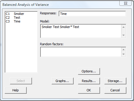
You might want to take particular note of the way we specify the interaction between smoking status and the type of test in Minitab, namely, as Smoker*Test.
We select OK, and the resulting output appears in the Session Window.

Here's what the output looks like with the row pertaining to the interaction term highlighted in yellow:

ANOVA, Time versus Smoker, Test
Factor	Type	Levels	Values
Smoker	fixed	3	1, 2, 3
Test	fixed	3	1, 2, 3

Analysis of Variance for Time
Source	DF	SS	MS	F	P
Smoker	2	84.899	42.449	12.90	0.000
Test	2	298.072	149.036	45.28	0.000
Smoker*Test	4	2.815	0.704	0.21	0.927
Error	18	59.247	3.291
Total	26	445.032

S = 1.81424 R-Sq = 86.69% R-Sq (adj) = 80.77%

As you can see, the P-value, 0.927, is very large. We do not reject the null hypothesis that the interaction terms are all zero. That is, there is insufficient evidence at the 0.05 level to conclude that there is an interaction between smoking history and the type of stress test.

Now, testing whether or not smoking history has an effect on the timing of maximum oxygen uptake involves testing the null hypothesis:

$H_{0} : α_{1} = α_{2} = α_{3} = 0$

against all of the possible alternatives. Here's what the output looks like with the row pertaining to the smoking history term highlighted in yellow:

ANOVA, Time versus Smoker, Test
Factor	Type	Levels	Values
Smoker	fixed	3	1, 2, 3
Test	fixed	3	1, 2, 3

Analysis of Variance for Time
Source	DF	SS	MS	F	P
Smoker	2	84.899	42.449	12.90	0.000
Test	2	298.072	149.036	45.28	0.000
Smoker*Test	4	2.815	0.704	0.21	0.927
Error	18	59.247	3.291
Total	26	445.032

S = 1.81424 R-Sq = 86.69% R-Sq (adj) = 80.77%

As you can see, the P-value is very small (< 0.001). We reject the null hypothesis that the smoking history parameters are all zero. That is, there is sufficient evidence at the 0.05 level to conclude that smoking history has an effect on the timing of maximum oxygen uptake.

Now, testing whether or not the type of stress test has an effect on the timing of maximum oxygen uptake involves testing the null hypothesis:

$H_{0} : β_{1} = β_{2} = β_{3} = 0$

against all of the possible alternatives. Here's what the output looks like with the row pertaining to the type of stress test term highlighted in yellow:

ANOVA, Time versus Smoker, Test
Factor	Type	Levels	Values
Smoker	fixed	3	1, 2, 3
Test	fixed	3	1, 2, 3

Analysis of Variance for Time
Source	DF	SS	MS	F	P
Smoker	2	84.899	42.449	12.90	0.000
Test	2	298.072	149.036	45.28	0.000
Smoker*Test	4	2.815	0.704	0.21	0.927
Error	18	59.247	3.291
Total	26	445.032

S = 1.81424 R-Sq = 86.69% R-Sq (adj) = 80.77%

As you can see, again, the P-value is very small (< 0.001). We reject the null hypothesis that the stress test parameters are all zero. That is, there is sufficient evidence at the 0.05 level to conclude that the type of stress test has an effect on the timing of maximum oxygen uptake.

In summary, based on these data, the physiologist can conclude that there appears to be an effect due to smoking history and the type of stress test, but that the data do not suggest that the two factors interact in any way.

Note!

We were able to include an interaction term in our model in the previous example, because we had multiple observations (three, to be exact) falling in each of the cells. That is, if there is only one observation in each cell, we cannot include an interaction term in our model.

Lesson 15: Tests Concerning Regression and Correlation

Overview

In lessons 35 and 36, we learned how to calculate point and interval estimates of the intercept and slope parameters, $α$ and $β$ , of a simple linear regression model:

$Y_{i} = α + β (x_{i} - \bar{x}) + ϵ_{i}$

with the random errors $ϵ_{i}$ following a normal distribution with mean 0 and variance $σ^{2}$ . In this lesson, we'll learn how to conduct a hypothesis test for testing the null hypothesis that the slope parameter equals some value, $β_{0}$ , say. Specifically, we'll learn how to test the null hypothesis $H_{0} : β = β_{0}$ using a $t$ -statistic.

Now, perhaps it is not a point that has been emphasized yet, but if you take a look at the form of the simple linear regression model, you'll notice that the response $Y$ 's are denoted using a capital letter, while the predictor $x$ 's are denoted using a lowercase letter. That's because, in the simple linear regression setting, we view the predictors as fixed values, whereas we view the responses as random variables whose possible values depend on the population $x$ from which they came. Suppose instead that we had a situation in which we thought of the pair $(X_{i}, Y_{i})$ as being a random sample, $i = 1, 2, \dots, n$ , from a bivariate normal distribution with parameters $μ_{X}$ , $μ_{Y}$ , $σ_{X}^{2}$ , $σ_{Y}^{2}$ and $ρ$ . Then, we might be interested in testing the null hypothesis $H_{0} : ρ = 0$ , because we know that if the correlation coefficient is 0, then $X$ and $Y$ are independent random variables. For this reason, we'll learn, not one, but three (!) possible hypothesis tests for testing the null hypothesis that the correlation coefficient is 0. Then, because we haven't yet derived an interval estimate for the correlation coefficient, we'll also take the time to derive an approximate confidence interval for $ρ$ .

15.1 - A Test for the Slope

Once again we've already done the bulk of the theoretical work in developing a hypothesis test for the slope parameter $β$ of a simple linear regression model when we developed a $(1 - α) 100 %$ confidence interval for $β$ . We had shown then that:

$T = \frac{\hat{β} - β}{\sqrt{\frac{M S E}{\sum (x_{i} - \bar{x})^{2}}}}$

follows a $t_{n - 2}$ distribution. Therefore, if we're interested in testing the null hypothesis:

$H_{0} : β = β_{0}$

against any of the alternative hypotheses:

$H_{A} : β \neq β_{0}$ , $H_{A} : β < β_{0}$ , $H_{A} : β > β_{0}$

we can use the test statistic:

$t = \frac{\hat{β} - β_{0}}{\sqrt{\frac{M S E}{\sum (x_{i} - \bar{x})^{2}}}}$

and follow the standard hypothesis testing procedures. Let's take a look at an example.

Example 15-1

In alligators' natural habitat, it is typically easier to observe the length of an alligator than it is the weight. This data set contains the log weight ( $y$ ) and log length ( $x$ ) for 15 alligators captured in central Florida. A scatter plot of the data suggests that there is a linear relationship between the response $y$ and the predictor $x$ . Therefore, a wildlife researcher is interested in fitting the linear model: ^[2] ^[3]

$Y_{i} = α + β x_{i} + ϵ_{i}$

to the data. She is particularly interested in testing whether there is a relationship between the length and weight of alligators. At the $α = 0.05$ level, perform a test of the null hypothesis $H_{0} : β = 0$ against the alternative hypothesis $H_{A} : β \neq 0$ .

Answer

The easiest way to perform the hypothesis test is to let Minitab do the work for us! Under the Stat menu, selecting Regression, and then Regression, and specifying the response logW (for log weight) and the predictor logL (for log length), we get:

The regression equation is
logW = - 8.48 + 3.43 logL

Predictor	Coef	SE Coef	T	P
Constant	-8.4761	0.5007	-16.93	0.000
logL	3.4311	0.1330	25.80	0.000

Analysis of Variance

Source	DF	SS	MS	F	P
Regression	1	10.064	10.064	665.81	0.000
Residual Error	13	0.196	0.015
Total	14	10.260

Easy as pie! Minitab tells us that the test statistic is $t = 25.80$ (in blue) with a $p$ -value (0.000) that is less than 0.001. Because the $p$ -value is less than 0.05, we reject the null hypothesis at the 0.05 level. There is sufficient evidence to conclude that the slope parameter does not equal 0. That is, there is sufficient evidence, at the 0.05 level, to conclude that there is a linear relationship, among the population of alligators, between the log length and log weight.

Of course, since we are learning this material for just the first time, perhaps we could go through the calculation of the test statistic at least once. Letting Minitab do some of the dirtier calculations for us, such as calculating:

$\sum (x_{i} - \bar{x})^{2} = 0.8548$

as well as determining that $M S E = 0.015$ and that the slope estimate = 3.4311, we get:

$t = \frac{\hat{β} - β_{0}}{\sqrt{\frac{M S E}{\sum (x_{i} - \bar{x})^{2}}}} = \frac{3.4311 - 0}{\sqrt{0.015 / 0.8548}} = 25.9$

which is the test statistic that Minitab calculated... well, with just a bit of round-off error.

15.2 - Three Tests for Rho

The hypothesis test for the slope $β$ that we developed on the previous page was developed under the assumption that a response $Y$ is a linear function of a nonrandom predictor $x$ . This situation occurs when the researcher has complete control of the values of the variable $x$ . For example, a researcher might be interested in modeling the linear relationship between the temperature $x$ of an oven and the moistness $y$ of chocolate chip muffins. In this case, the researcher sets the oven temperatures (in degrees Fahrenheit) to 350, 360, 370, and so on, and then observes the values of the random variable $Y$ , that is, the moistness of the baked muffins. In this case, the linear model:

$Y_{i} = α + β x_{i} + ϵ_{i}$

implies that the average moistness:

$E (Y) = α + β x$

is a linear function of the temperature setting.

There are other situations, however, in which the variable $x$ is not nonrandom (yes, that's a double negative!), but rather an observed value of a random variable $X$ . For example, a fisheries researcher may want to relate the age $Y$ of a sardine to its length $X$ . If a linear relationship could be established, then in the future fisheries researchers could predict the age of a sardine simply by measuring its length. In this case, the linear model:

$Y_{i} = α + β x_{i} + ϵ_{i}$

implies that the average age of a sardine, given its length is $X = x$ :

$E (Y | X = x) = α + β x$

is a linear function of the length. That is, the conditional mean of $Y$ given $X = x$ is a linear function. Now, in this second situation, in which both $X$ and $Y$ are deemed random, we typically assume that the pairs $(X_{1}, Y_{1}), (X_{2}, Y_{2}), \dots, (X_{n}, Y_{n})$ are a random sample from a bivariate normal distribution with means $μ_{X}$ and $μ_{Y}$ , variances $σ_{X}^{2}$ and $σ_{Y}^{2}$ , and correlation coefficient $ρ$ . If that's the case, it can be shown that the conditional mean:

$E (Y | X = x) = α + β x$

must be of the form:

$E (Y | X = x) = (μ_{Y} - ρ \frac{σ_{Y}}{σ_{X}} μ_{X}) + (ρ \frac{σ_{Y}}{σ_{X}}) x$

That is:

$β = ρ \frac{σ_{Y}}{σ_{X}}$

Now, for the case where $(X_{i}, Y_{i})$ has a bivariate distribution, the researcher may not necessarily be interested in estimating the linear function:

$E (Y | X = x) = α + β x$

but rather simply knowing whether $X$ and $Y$ are independent. In STAT 414, we've learned that if $(X_{i}, Y_{i})$ follows a bivariate normal distribution, then testing for the independence of $X$ and $Y$ is equivalent to testing whether the correlation coefficient $ρ$ equals 0. We'll now work on developing three different hypothesis tests for testing $H_{0} : ρ = 0$ assuming $(X_{i}, Y_{i})$ follows a bivariate normal distribution.

A T-Test for Rho

Given our wordy prelude above, this test may be the simplest of all of the tests to develop. That's because we argued above that if $(X_{i}, Y_{i})$ follows a bivariate normal distribution, and the conditional mean is a linear function:

$E (Y | X = x) = α + β x$

then:

$β = ρ \frac{σ_{Y}}{σ_{X}}$

That suggests, therefore, that testing for $H_{0} : ρ = 0$ against any of the alternative hypotheses $H_{A} : ρ \neq 0$ , $H_{A} : ρ > 0$ and $H_{A} : ρ < 0$ is equivalent to testing $H_{0} : β = 0$ against the corresponding alternative hypothesis $H_{A} : β \neq 0$ , $H_{A} : β < 0$ and $H_{A} : β > 0$ . That is, we can simply compare the test statistic:

$t = \frac{\hat{β} - 0}{\sqrt{M S E / \sum (x_{i} - \bar{x})^{2}}}$

to a $t$ distribution with $n - 2$ degrees of freedom. It should be noted, though, that the test statistic can be instead written as a function of the sample correlation coefficient:

$R = \frac{\frac{1}{n - 1} \sum_{i = 1}^{n} (X_{i} - \bar{X}) (Y_{i} - \bar{Y})}{\sqrt{\frac{1}{n - 1} \sum_{i = 1}^{n} (X_{i} - \bar{X})^{2}} \sqrt{\frac{1}{n - 1} \sum_{i = 1}^{n} (Y_{i} - \bar{Y})^{2}}} = \frac{S_{x y}}{S_{x} S_{y}}$

That is, the test statistic can be alternatively written as:

$t = \frac{r \sqrt{n - 2}}{\sqrt{1 - r^{2}}}$

and because of its algebraic equivalence to the first test statistic, it too follows a $t$ distribution with $n - 2$ degrees of freedom. Huh? How are the two test statistics algebraically equivalent? Well, if the following two statements are true:

$\hat{β} = \frac{\frac{1}{n - 1} \sum_{i = 1}^{n} (X_{i} - \bar{X}) (Y_{i} - \bar{Y})}{\frac{1}{n - 1} \sum_{i = 1}^{n} (X_{i} - \bar{X})^{2}} = \frac{S_{x y}}{S_{x}^{2}} = R \frac{S_{y}}{S_{x}}$
$M S E = \frac{\sum_{i = 1}^{n} (Y_{i} - {\hat{Y}}_{i})^{2}}{n - 2} = \frac{\sum_{i = 1}^{n} {[Y_{i} - (\bar{Y} + \frac{S_{x y}}{S_{x}^{2}} (X_{i} - \bar{X}))]}^{2}}{n - 2} = \frac{(n - 1) S_{Y}^{2} (1 - R^{2})}{n - 2}$

then simple algebra illustrates that the two test statistics are indeed algebraically equivalent:

$t = \frac{\hat{β}}{\sqrt{\frac{M S E}{\sum (x_{i} - \bar{x})^{2}}}} = \frac{r (\frac{S_{y}}{S_{x}})}{\sqrt{\frac{(n - 1) S_{y}^{2} (1 - r^{2})}{(n - 2) (n - 1) S_{x}^{2}}}} = \frac{r \sqrt{n - 2}}{\sqrt{1 - r^{2}}}$

Now, for the veracity of those two statements? Well, they are indeed true. The first one requires just some simple algebra. The second one requires a bit of trickier algebra that you'll soon be asked to work through for homework.

An R-Test for Rho

It would be nice to use the sample correlation coefficient $R$ as a test statistic to test more general hypotheses about the population correlation coefficient:

$H_{0} : ρ = ρ_{0}$

but the probability distribution of $R$ is difficult to obtain. It turns out though that we can derive a hypothesis test using just $R$ provided that we are interested in testing the more specific null hypothesis that $X$ and $Y$ are independent, that is, for testing $H_{0} : ρ = 0$ .

Theorem

Provided that $ρ = 0$ , the probability density function of the sample correlation coefficient $R$ is:

$g (r) = \frac{Γ [(n - 1) / 2]}{Γ (1 / 2) Γ [(n - 2) / 2]} (1 - r^{2})^{(n - 4) / 2}$

over the support $- 1 < r < 1$ .

Proof

We'll use the distribution function technique, in which we first find the cumulative distribution function $G (r)$ , and then differentiate it to get the desired probability density function $g (r)$ . The cumulative distribution function is:

$G (r) = P (R \leq r) = P (\frac{R \sqrt{n - 2}}{\sqrt{1 - R^{2}}} \leq \frac{r \sqrt{n - 2}}{\sqrt{1 - r^{2}}}) = P (T \leq \frac{r \sqrt{n - 2}}{\sqrt{1 - r^{2}}})$

The first equality is just the definition of the cumulative distribution function, while the second and third equalities come from the definition of the $T$ statistic as a function of the sample correlation coefficient $R$ . Now, using what we know of the p.d.f. $h (t)$ of a $T$ random variable with $n - 2$ degrees of freedom, we get:

$G (r) = \int_{- \infty}^{\frac{r \sqrt{n - 2}}{\sqrt{1 - r^{2}}}} h (t) d t = \int_{- \infty}^{\frac{r \sqrt{n - 2}}{\sqrt{1 - r^{2}}}} \frac{Γ [(n - 1) / 2]}{Γ (1 / 2) Γ [(n - 2) / 2]} \frac{1}{\sqrt{n - 2}} {(1 + \frac{t^{2}}{n - 2})}^{- \frac{(n - 1)}{2}} d t$

Now, it's just a matter of taking the derivative of the c.d.f. $G (r)$ to get the p.d.f. $g (r)$ ). Using the Fundamental Theorem of Calculus, in conjunction with the chain rule, we get:

$g (r) = h (\frac{r \sqrt{n - 2}}{\sqrt{1 - r^{2}}}) \frac{d}{d r} (\frac{r \sqrt{n - 2}}{\sqrt{1 - r^{2}}})$

Focusing first on the derivative part of that equation, using the quotient rule, we get:

$\frac{d}{d r} [\frac{r \sqrt{n - 2}}{\sqrt{1 - r^{2}}}] = \frac{(1 - r^{2})^{1 / 2} \cdot \sqrt{n - 2} - r \sqrt{n - 2} \cdot \frac{1}{2} (1 - r^{2})^{- 1 / 2} \cdot - 2 r}{(\sqrt{1 - r^{2}})^{2}}$

Simplifying, we get:

$\frac{d}{d r} [\frac{r \sqrt{n - 2}}{\sqrt{1 - r^{2}}}] = \sqrt{n - 2} [\frac{(1 - r^{2})^{1 / 2} + r^{2} (1 - r^{2})^{- 1 / 2}}{1 - r^{2}}]$

Now, if we multiply by 1 in a special way, that is, this way:

$\frac{d}{d r} [\frac{r \sqrt{n - 2}}{\sqrt{1 - r^{2}}}] = \sqrt{n - 2} [\frac{(1 - r^{2})^{1 / 2} + r^{2} (1 - r^{2})^{- 1 / 2}}{1 - r^{2}}] (\frac{(1 - r^{2})^{1 / 2}}{(1 - r^{2})^{1 / 2}})$

and then simplify, we get:

$\frac{d}{d r} [\frac{r \sqrt{n - 2}}{\sqrt{1 - r^{2}}}] = \sqrt{n - 2} [\frac{1 - r^{2} + r^{2}}{(1 - r^{2})^{3 / 2}}] = \sqrt{n - 2} (1 - r^{2})^{- 3 / 2}$

Now, looking back at $g (r)$ , let's work on the $h (.)$ part. Replacing the function in the one place where a t appears in the p.d.f. of a $T$ random variable with $n - 2$ degrees of freedom, we get:

$h (\frac{r \sqrt{n - 2}}{\sqrt{1 - r^{2}}}) = \frac{Γ (\frac{n - 1}{2})}{Γ (\frac{1}{2}) Γ (\frac{n - 2}{2})} (\frac{1}{\sqrt{n - 2}}) {[1 + \frac{{(\frac{r \sqrt{n - 2}}{\sqrt{1 - r^{2}}})}^{2}}{n - 2}]}^{- \frac{n - 1}{2}}$

Canceling a few things out we get:

$h (\frac{r \sqrt{n - 2}}{\sqrt{1 - r^{2}}}) = \frac{Γ [(n - 1) / 2]}{Γ (1 / 2) Γ [(n - 2) / 2]} \cdot \frac{1}{\sqrt{n - 2}} {(1 + \frac{r^{2}}{1 - r^{2}})}^{- \frac{(n - 1)}{2}}$

Now, because:

${(1 + \frac{r^{2}}{1 - r^{2}})}^{- \frac{(n - 1)}{2}} = {(\frac{1 - r^{2} + r^{2}}{1 - r^{2}})}^{- \frac{(n - 1)}{2}} = {(\frac{1}{1 - r^{2}})}^{- \frac{(n - 1)}{2}} = (1 - r^{2})^{\frac{(n - 1)}{2}}$

we finally get:

$h (\frac{r \sqrt{n - 2}}{\sqrt{1 - r^{2}}}) = \frac{Γ [(n - 1) / 2]}{Γ (1 / 2) Γ [(n - 2) / 2]} \cdot \frac{1}{\sqrt{n - 2}} (1 - r^{2})^{\frac{(n - 1)}{2}}$

We're almost there! We just need to multiply the two parts together. Doing so, we get:

$g (r) = [\frac{Γ (\frac{n - 1}{2})}{Γ (\frac{1}{2}) Γ (\frac{n - 2}{2})} (\frac{1}{\sqrt{n - 2}}) (1 - r^{2})^{\frac{n - 1}{2}}] [\sqrt{n - 2} (1 - r^{2})^{- 3 / 2}]$

which simplifies to:

$g (r) = \frac{Γ [(n - 1) / 2]}{Γ (1 / 2) Γ [(n - 2) / 2]} (1 - r^{2})^{(n - 4) / 2}$

over the support $- 1 < r < 1$ , as was to be proved.

Now that we know the p.d.f. of $R$ , testing $H_{0} : ρ = 0$ against any of the possible alternative hypotheses just involves integrating $g (r)$ to find the critical value(s) to ensure that $α$ , the probability of a Type I error is small. For example, to test $H_{0} : ρ = 0$ against the alternative $H_{A} : ρ > 0$ , we find the value $r_{α} (n - 2)$ such that:

$P (R \geq r_{α} (n - 2)) = \int_{r_{α} (n - 2)}^{1} \frac{Γ [(n - 1) / 2]}{Γ (1 / 2) Γ [(n - 2) / 2]} (1 - r^{2})^{\frac{(n - 4)}{2}} d r = α$

Yikes! Do you have any interest in integrating that function? Well, me neither! That's why we'll instead use an $R$ Table, such as the one we have in Table IX at the back of our textbook.

An Approximate Z-Test for Rho

Okay, the derivation for this hypothesis test is going to be MUCH easier than the derivation for that last one. That's because we aren't going to derive it at all! We are going to simply state, without proof, the following theorem.

Theorem

The statistic:

$W = \frac{1}{2} \ln \frac{1 + R}{1 - R}$

follows an approximate normal distribution with mean $E (W) = \frac{1}{2} \ln \frac{1 + ρ}{1 - ρ}$ and variance $V a r (W) = \frac{1}{n - 3}$ .

The theorem, therefore, allows us to test the general null hypothesis $H_{0} : ρ = ρ_{0}$ against any of the possible alternative hypotheses comparing the test statistic:

$Z = \frac{\frac{1}{2} l n \frac{1 + R}{1 - R} - \frac{1}{2} l n \frac{1 + ρ_{0}}{1 - ρ_{0}}}{\sqrt{\frac{1}{n - 3}}}$

to a standard normal $N (0, 1)$ distribution.

What? We've looked at no examples yet on this page? Let's take care of that by closing with an example that utilizes each of the three hypothesis tests we derived above.

Example 15-2

An admissions counselor at a large public university was interested in learning whether freshmen calculus grades are independent of high school math achievement test scores. The sample correlation coefficient between the mathematics achievement test scores and calculus grades for a random sample of $n = 10$ college freshmen was deemed to be 0.84.

Does this observed sample correlation coefficient suggest, at the $α = 0.05$ level, that the population of freshmen calculus grades are independent of the population of high school math achievement test scores?

Answer

The admissions counselor is interested in testing:

$H_{0} : ρ = 0$ against $H_{A} : ρ \neq 0$

Using the $t$ -statistic we derived, we get:

$t = \frac{r \sqrt{n - 2}}{\sqrt{1 - r^{2}}} = \frac{0.84 \sqrt{8}}{\sqrt{1 - {0.84}^{2}}} = 4.38$

We reject the null hypothesis if the test statistic is greater than 2.306 or less than −2.306.

Because $t = 4.38 > 2.306$ , we reject the null hypothesis in favor of the alternative hypothesis. There is sufficient evidence at the 0.05 level to conclude that the population of freshmen calculus grades are not independent of the population of high school math achievement test scores.

Using the R-statistic, with 8 degrees of freedom, Table IX in the back of the book tells us to reject the null hypothesis if the absolute value of $R$ is greater than 0.6319. Because our observed $r = 0.84 > 0.6319$ , we again reject the null hypothesis in favor of the alternative hypothesis. There is sufficient evidence at the 0.05 level to conclude that freshmen calculus grades are not independent of high school math achievement test scores.

Using the approximate Z-statistic, we get:

$z = \frac{\frac{1}{2} l n (\frac{1 + 0.84}{1 - 0.84}) - \frac{1}{2} l n (\frac{1 + 0}{1 - 0})}{\sqrt{1 / 7}} = 3.23$

In this case, we reject the null hypothesis if the absolute value of $Z$ were greater than 1.96. It clearly is, and so we again reject the null hypothesis in favor of the alternative hypothesis. There is sufficient evidence at the 0.05 level to conclude that freshmen calculus grades are not independent of high school math achievement test scores.

15.3 - An Approximate Confidence Interval for Rho

To develop an approximate $(1 - α) 100 %$ confidence interval for $ρ$ , we'll use the normal approximation for the statistic $Z$ that we used on the previous page for testing $H_{0} : ρ = ρ_{0}$ .

Theorem

An approximate $(1 - α) 100 %$ confidence interval for $ρ$ is $L \leq ρ \leq U$ where:

$L = \frac{1 + R - (1 - R) exp (2 z_{α / 2} / \sqrt{n - 3})}{1 + R + (1 - R) exp (2 z_{α / 2} / \sqrt{n - 3})}$

and

$U = \frac{1 + R - (1 - R) exp (- 2 z_{α / 2} / \sqrt{n - 3})}{1 + R + (1 - R) exp (- 2 z_{α / 2} / \sqrt{n - 3})}$

Proof

We previously learned that:

$Z = \frac{\frac{1}{2} l n \frac{1 + R}{1 - R} - \frac{1}{2} l n \frac{1 + ρ}{1 - ρ}}{\sqrt{\frac{1}{n - 3}}}$

follows at least approximately a standard normal $N (0, 1)$ distribution. So, we can do our usual trick of starting with a probability statement:

$P (- z_{α / 2} \leq \frac{\frac{1}{2} l n \frac{1 + R}{1 - R} - \frac{1}{2} l n \frac{1 + ρ}{1 - ρ}}{\sqrt{\frac{1}{n - 3}}} \leq z_{α / 2}) \approx 1 - α$

and manipulating the quantity inside the parentheses:

$- z_{α / 2} \leq \frac{\frac{1}{2} l n \frac{1 + R}{1 - R} - \frac{1}{2} l n \frac{1 + ρ}{1 - ρ}}{\sqrt{\frac{1}{n - 3}}} \leq z_{α / 2}$

to get ..... can you fill in the details?! ..... the formula for a $(1 - α) 100 %$ confidence interval for $ρ$ :

$L \leq ρ \leq U$

where:

$L = \frac{1 + R - (1 - R) exp (2 z_{α / 2} / \sqrt{n - 3})}{1 + R + (1 - R) exp (2 z_{α / 2} / \sqrt{n - 3})}$ and $U = \frac{1 + R - (1 - R) exp (- 2 z_{α / 2} / \sqrt{n - 3})}{1 + R + (1 - R) exp (- 2 z_{α / 2} / \sqrt{n - 3})}$

as was to be proved!

Example 15-2 (Continued)

Estimate the population correlation coefficient $ρ$ with 95% confidence.

Answer

Because we are interested in a 95% confidence interval, we use $z_{0.025} = 1.96$ . Therefore, the lower limit of an approximate 95% confidence interval for $ρ$ is:

$L = \frac{1 + 0.84 - (1 - 0.84) exp (2 (1.96) / \sqrt{10 - 3})}{1 + 0.84 + (1 - 0.84) exp (2 (1.96) / \sqrt{10 - 3})} = 0.447$

and the upper limit of an approximate 95% confidence interval for $ρ$ is:

$U = \frac{1 + 0.84 - (1 - 0.84) exp (- 2 (1.96) / \sqrt{10 - 3})}{1 + 0.84 + (1 - 0.84) exp (- 2 (1.96) / \sqrt{10 - 3})} = 0.961$

We can be (approximately) 95% confident that the correlation between the population of high school mathematics achievement test scores and freshmen calculus grades is between 0.447 and 0.961. (Not a particularly useful interval, I might say! It might behoove the admissions counselor to collect data on a larger sample, so that he or she can obtain a narrower confidence interval.)

^[1]	Link
↥	Has Tooltip/Popover
	Toggleable Visibility

Brand1	Brand2	Brand3	Brand4	Brand5
194	189	185	183	195
184	204	183	193	197
189	190	186	184	194
189	190	183	186	202
188	189	179	194	200
186	207	191	199	211
195	203	188	196	203
186	193	196	188	206
183	181	189	193	202
188	206	194	196	195

Brand1	Brand2	Brand3	Brand4	Brand5
194	189	185	183	195
184	204	183	193	197
189	190	186	184	194
189	190	183	186	202
188	189	179	194	200
186	207	191	199	211
195	203	188	196	203
186	193	196	188	206
183	181	189	193	202
188	206	194	196	195

Section 2: Hypothesis Testing

Lesson 9: Tests About Proportions

9.1 - The Basic Idea

Example 9-1

Answer

Example (continued)

Answer

Possible Errors

9.2 - More Examples

Example 9-2

Answer

Example 9-3

Answer

9.3 - The P-Value Approach

Example 9-4

Answer

Example 9-4 (continued)

Answer

Example 9-4 (continued)

Answer

Example 9-4 (continued)

Answer

Note!

Answer

9.4 - Comparing Two Proportions

Example 9-5

Answer

Proof

Example 9-5 (continued)

Answer

Note!

9.5 - Using Minitab

Hypothesis Test for a Single Proportion

Hypothesis Test for Comparing Two Proportions

Lesson 10: Tests About One Mean

Overview

10.1 - Z-Test: When Population Variance is Known

Example 10-1

Answer

10.2 - T-Test: When Population Variance is Unknown

Example 10-2

Answer

10.3 - Paired T-Test

Example 10-3

Answer

10.4 - Using Minitab

Z-Test for a Single Mean

T-test for a Single Mean

One Sample T: Diff

Lesson 11: Tests of the Equality of Two Means

Overview

11.1 - When Population Variances Are Equal

Example 11-1

Answer

Two-Sample T: For Fastest

11.2 - When Population Variances Are Not Equal

Example 11-1 (Continued)

Answer

Two-Sample T: For Fastest

11.3 - Using Minitab

When the Data are Entered in Two Columns

When the Data are Entered in One Column, and a Grouping Variable in a Second Column

Two-Sample T: For Prey

Lesson 12: Tests for Variances

12.1 - One Variance

Example 12-1

Answer

Answer

12.2 - Two Variances

Example 12-2

Answer

12.3 - Using Minitab

Hypothesis Test for One Variance

Hypothesis Test for Two Variances

Test and CI for Two Variances

Lesson 13: One-Factor Analysis of Variance

13.1 - The Basic Idea

Example 13-1

Answer

Example 13-2

Minitab^®

Brand1	Brand2	Brand3	Brand4	Brand5
194	189	185	183	195
184	204	183	193	197
189	190	186	184	194
189	190	183	186	202
188	189	179	194	200
186	207	191	199	211
195	203	188	196	203
186	193	196	188	206
183	181	189	193	202
188	206	194	196	195