Section 3: Nonparametric Methods
Section 3: Nonparametric Methods
In the previous sections, all of the methods we derived were based on making some sort of underlying assumptions about the data − for example, "the data are normally distributed," or the "population variances are equal." How do we go about using our data to answer our scientific questions if the assumptions on which our methods are based don't hold? That's what we'll tackle in this section. Specifically, we will:
- learn how to use the chi-square goodness of fit test to test whether random categorical variables follow a particular probability distribution
- learn how to use the chi-square test for testing whether two or more multinomial distributions are equal
- learn how to use the chi-square test to test whether two (or more) random categorical variables are independent
- define, determine, and use order statistics to draw conclusions about a median, as well as other percentiles
- learn how to use the Wilcoxon test to conduct a hypothesis test for the median of a population
- learn how to use a run test to test the equality of two distribution functions
- learn how to use a run test to test for the randomness of a sequence of events
- learn how to use the Kolmogorov-Smirnov goodness-of-fit test to test how well an empirical distribution function fits a hypothesized distribution function
- learn how to use resampling methods to find approximate distributions of statistics that are used to make statistical inference
Lesson 16: Chi-Square Goodness-of-Fit Tests
Lesson 16: Chi-Square Goodness-of-Fit TestsSuppose the Penn State student population is 60% female and 40%, male. Then, if a sample of 100 students yields 53 females and 47 males, can we conclude that the sample is (random and) representative of the population? That is, how "good" do the data "fit" the probability model? As the title of the lesson suggests, that's the kind of question that we will answer in this lesson.
16.1 - The General Approach
16.1 - The General ApproachExample 16-1

As is often the case, we'll motivate the methods of this lesson by way of example. Specifically, we'll return to the question posed in the introduction to this lesson.
Suppose the Penn State student population is 60% female and 40%, male. Then, if a sample of 100 students yields 53 females and 47 males, can we conclude that the sample is (random and) representative of the population? That is, how "good" do the data "fit" the assumed probability model of 60% female and 40% male?
Answer
Testing whether there is a "good fit" between the observed data and the assumed probability model amounts to testing:
\(H_0 : p_F =0.60\)
\(H_A : p_F \ne 0.60\)
Now, letting \(Y_1\) denote the number of females selected, we know that \(Y_1\) follows a binomial distribution with n trials and probability of success \(p_1\). That is:
\(Y_1 \sim b(n,p_1)\)
Therefore, the expected value and variance of \(Y_1\) are, respectively:
\(E(Y_1)=np_1\) and \(Var (Y_1) =np_1(1-p_1)\)
And, letting \(Y_2\) denote the number of males selected, we know that \(Y_2 = n − Y_1\) follows a binomial distribution with n trials and probability of success \(p_2\). That is:
\(Y_2 = n-Y_1 \sim (b(n,p_2)=b(n,1-p_1)\)
Therefore, the expected value and variance of \(Y_2\) are, respectively:
\(E(Y_2)=n(1-p_1)=np_2\) and \(Var(Y_2)=n(1-p_1)(1-(1-p_1))=np_1(1-p_1)=np_2(1-p_2)\)
Now, for large samples (\(np_1 ≥ 5\) and \(n(1 − p_1) ≥ 5)\), the Central Limit Theorem yields the normal approximation to the binomial distribution. That is:
\(Z=\dfrac{(Y_1-np_1)}{\sqrt{np_1(1-p_1)}}\)
follows, at least approximately, the standard normal N(0,1) distribution. Therefore, upon squaring Z, we get that:
\(Z^2=Q_1=\dfrac{(Y_1-np_1)^2}{np_1(1-p_1)}\)
follows an approximate chi-square distribution with one degree of freedom. Now, we could stop there. But, that's not typically what is done. Instead, we can rewrite \(Q_1\) a bit. Let's start by multiplying \(Q_1\) by 1 in a special way, that is, by multiplying it by \(\left( \left( 1 − p_1 \right) + p_1 \right)\):
\(Q_1=\dfrac{(Y_1-np_1)^2}{np_1(1-p_1)} \times ((1-p_1)+p_1)\)
Then, distributing the "1" across the numerator, we get:
\(Q_1=\dfrac{(Y_1-np_1)^2(1-p_1)}{np_1(1-p_1)}+\dfrac{(Y_1-np_1)^2p_1}{np_1(1-p_1)}\)
which simplies to:
\(Q_1=\dfrac{(Y_1-np_1)^2}{np_1}+\dfrac{(Y_1-np_1)^2}{n(1-p_1)}\)
Now, taking advantage of the fact that \(Y_1 = n − Y_2\) and \(p_1 = 1 − p_2\), we get:
\(Q_1=\dfrac{(Y_1-np_1)^2}{np_1}+\dfrac{(n-Y_2-n(1-p_2))^2}{np_2}\)
which simplifies to:
\(Q_1=\dfrac{(Y_1-np_1)^2}{np_1}+\dfrac{(-(Y_2-np_2))^2}{np_2}\)
Just one more thing to simplify before we're done:
\(Q_1=\dfrac{(Y_1-np_1)^2}{np_1}+\dfrac{(Y_2-np_2)^2}{np_2}\)
In summary, we have rewritten \(Q_1\) as:
\( Q_1=\sum_{i=1}^{2}\dfrac{(Y_i-np_i)^2}{np_i}=\sum_{i=1}^{2}\dfrac{(\text{OBSERVED }-\text{ EXPECTED})^2}{EXPECTED} \)
We'll use this form of \(Q_1\), and the fact that \(Q_1\) follows an approximate chi-square distribution with one degree of freedom, to conduct the desired hypothesis test.
Before we return to solving the problem posed by our example, a couple of points are worthy of emphasis.
- First, \(Q_1\) has only one degree of freedom, since there is only one independent count, namely \(Y_1\). Once \(Y_1\) is known, the value of \(Y_2 = n − Y_1\) immediately follows.
- Note that the derived approach requires the Central Limit Theorem to kick in. The general rule of thumb is that the expected number of successes must be at least 5 (that is, \(np_1 ≥ 5\)) and the expected number of failures must be at least 5 (that is, \(n(1−p_1) ≥ 5\)).
- The statistic \(Q_1\) will be large if the observed counts are very different from the expected counts. Therefore, we must reject the null hypothesis \(H_0\) if \(Q_1\) is large. How large is large? Large is determined by the values of a chi-square random variable with one degree of freedom, which can be obtained either from a statistical software package, such as Minitab or SAS or from a standard chi-square table, such as the one in the back of our textbook.
- The statistic \(Q_1\) is called the chi-square goodness-of-fit statistic.
Example 16-2

Suppose the Penn State student population is 60% female and 40%, male. Then, if a sample of 100 students yields 53 females and 47 males, can we conclude that the sample is (random and) representative of the population? Use the chi-square goodness-of-fit statistic to test the hypotheses:
\(H_0 : p_F =0.60\)
\(H_A : p_F \ne 0.60\)
using a significance level of \(\alpha = 0.05\).
Answer
The value of the test statistic \(Q_1\) is:
\(Q_1=\dfrac{(53-60)^2}{60}+\dfrac{(47-40)^2}{40}=2.04\)
We should reject the null hypothesis if the observed number of counts is very different from the expected number of counts, that is if \(Q_1\) is large. Because \(Q_1\) follows a chi-square distribution with one degree of freedom, we should reject the null hypothesis, at the 0.05 level, if:
\(Q_1 \ge \chi_{0.05, 1}^{2}=3.84\)
Because:
\(Q_1=2.04 < 3.84\)
we do not reject the null hypothesis. There is not enough evidence at the 0.05 level to conclude that the data don't fit the assumed probability model.
As an aside, it is interesting to note the relationship between using the chi-square goodness of fit statistic \(Q_1\) and the Z-statistic we've previously used for testing a null hypothesis about a proportion. In this case:
\( Z=\dfrac{0.53-0.60}{\sqrt{\frac{(0.60)(0.40)}{100}}}=-1.428 \)
which, you might want to note that, if we square it, we get the same value as we did for \(Q_1\):
\(Q_1=Z^2 =(-1.428)^2=2.04\)
as we should expect. The Z-test for a proportion tells us that we should reject if:
\(|Z| \ge 1.96 \)
Well, again, if we square it, we should see that that's equivalent to rejecting if:
\(Q_1 \ge (1.96)^2 =3.84\)
And not surprisingly, the P-values obtained from the two approaches are identical. The P-value for the chi-square goodness-of-fit test is:
\(P=P(\chi_{(1)}^{2} > 2.04)=0.1532\)
while the P-value for the Z-test is:
\(P=2 \times P(Z>1.428)=2(0.0766)=0.1532\)
Identical, as we should expect!
16.2 - Extension to K Categories
16.2 - Extension to K CategoriesThe work on the previous page is all well and good if your probability model involves just two categories, which as we have seen, reduces to conducting a test for one proportion. What happens if our probability model involves three or more categories? It takes some theoretical work beyond the scope of this course to show it, but the chi-square statistic that we derived on the previous page can be extended to accommodate any number of k categories.
The Extension

Suppose an experiment can result in any of k mutually exclusive and exhaustive outcomes, say \(A_1, A_2, \dots, A_k\). If the experiment is repeated n independent times, and we let \(p_i = P(A_i)\) and \(Y_i\) = the number of times the experiment results in \(A_i, i = 1, \dots, k\), then we can summarize the number of observed outcomes and the number of expected outcomes for each of the k categories in a table as follows:
| Categories | 1 | 2 | . . . | \(k - 1\) | \(k\) |
|---|---|---|---|---|---|
| Observed | \(Y_1\) | \(Y_2\) | . . . | \(Y_{k - 1}\) | \(n - Y_1 - Y_2 - . . . - Y_{k - 1}\) |
| Expected | \(np_1\) | \(np_2\) | . . . | \(np_{k - 1}\) | \(np_k\) |
Karl Pearson showed that the chi-square statistic Q_k−1 defined as:
\[Q_{k-1}=\sum_{i=1}^{k}\frac{(Y_i - np_i)^2}{np_i} \]
follows approximately a chi-square random variable with k−1 degrees of freedom. Let's try it out on an example.
Example 16-3

A particular brand of candy-coated chocolate comes in five different colors that we shall denote as:
- \(A_1 = \text{{brown}}\)
- \(A_2 = \text{{yellow}}\)
- \(A_3 = \text{{orange}}\)
- \(A_4 = \text{{green}}\)
- \(A_5 = \text{{coffee}}\)
Let \(p_i\) equal the probability that the color of a piece of candy selected at random belongs to \(A_i\), for \(i = 1, 2 3, 4, 5\). Test the following null and alternative hypotheses:
\(H_0 : p_{Br}=0.4,p_{Y}=0.2,p_{O}=0.2,p_{G}=0.1,p_{C}=0.1 \)
\(H_A : p_{i} \text{ not specified in null (many possible alternatives) } \)
using a random sample of n = 580 pieces of candy whose colors yielded the respective frequencies 224, 119, 130, 48, and 59. (This example comes from exercises 8.1-2 in the Hogg and Tanis (8th edition) textbook).
Answer
We can summarize the observed \((y_i)\) and expected \((np_i)\) counts in a table as follows:
| Categories | Brown | Yellow | Orange | Green | Coffee | Total |
|---|---|---|---|---|---|---|
| Observed \(y_i\) | 224 | 119 | 130 | 48 | 59 | 580 |
| Assumed \(H_0 (p_i)\) | 0.4 | 0.2 | 0.2 | 0.1 | 0.1 | 1.0 |
| Expected \(np_i\) | 232 | 116 | 116 | 58 | 58 | 580 |
where, for example, the expected number of brown candies is:
\(np_1 = 580(0.40) = 232\)
and the expected number of green candies is:
\(np_4 = 580(0.10) = 58\)
Once we have the observed and expected number of counts, the calculation of the chi-square statistic is straightforward. It is:
\(Q_4=\dfrac{(224-232)^2}{232}+d\frac{(119-116)^2}{116}+\dfrac{(130-116)^2}{116}+\dfrac{(48-58)^2}{58}+\dfrac{(59-58)^2}{58} \)
Simplifying, we get:
\(Q_4=\dfrac{64}{232}+\dfrac{9}{116}+\dfrac{196}{116}+\dfrac{100}{58}+\dfrac{1}{58}=3.784 \)
Because there are k = 5 categories, we have to compare our chi-square statistic \(Q_4\) to a chi-square distribution with k−1 = 5−1 = 4 degrees of freedom:
\(\text{Reject }H_0 \text{ if } Q_4\ge \chi_{4,0.05}^{2}=9.488\)
Because \(Q_4 = 3.784 < 9.488\), we fail to reject the null hypothesis. There is insufficient evidence at the 0.05 level to conclude that the distribution of the color of the candies differs from that specified in the null hypothesis.
By the way, this might be a good time to think about the practical meaning of the term "degrees of freedom." Recalling the example on the last page, we had two categories (male and female) and one degree of freedom. If we are sampling n = 100 people and 53 of them are female, then we absolutely must have 100−53 = 47 males. If we had instead 62 females, then we absolutely must have 100−62 = 38 males. That is, the number of females is the one number that is "free" to be any number, but once it is determined, then the number of males immediately follows. It is in this sense that we have "one degree of freedom."
With the example on this page, we have five categories of candies (brown, yellow, orange, green, coffee) and four degrees of freedom. If we are sampling n = 580 candies, and 224 are brown, 119 are yellow, 130 are orange, and 48 are green, then we absolutely must have 580−(224+119+130+48) = 59 coffee-colored candies. In this case, we have four numbers that are "free" to be any number, but once they are determined, then the number of coffee-colored candies immediately follows. It is in this sense that we have "four degrees of freedom."
16.3 - Unspecified Probabilities
16.3 - Unspecified ProbabilitiesFor the two examples that we've thus far considered, the probabilities were pre-specified. For the first example, we were interested in seeing if the data fit a probability model in which there was a 0.60 probability that a randomly selected Penn State student was female. In the second example, we were interested in seeing if the data fit a probability model in which the probabilities of selecting a brown, yellow, orange, green, and coffee-colored candy was 0.4, 0.2, 0.2, 0.1, and 0.1, respectively. That is, we were interested in testing specific probabilities:
\(H_0 : p_{B}=0.40,p_{Y}=0.20,p_{O}=0.20,p_{G}=0.10,p_{C}=0.10 \)
Someone might be also interested in testing whether a data set follows a specific probability distribution, such as:
\(H_0 : X \sim b(n, 1/2)\)
What if the probabilities aren't pre-specified though? That is, suppose someone is interested in testing whether a random variable is binomial, but with an unspecified probability of success:
\(H_0 : X \sim b(n, p)\)
Can we still use the chi-square goodness-of-fit statistic? The short answer is yes... with just a minor modification.
Example 16-4

Let X denote the number of heads when four dimes are tossed at random. One hundred repetitions of this experiment resulted in 0, 1, 2, 3, and 4 heads being observed on 8, 17, 41, 30, and 4 trials, respectively. Under the assumption that the four dimes are independent, and the probability of getting a head on each coin is p, the random variable X is b(4, p). In light of the observed data, is b(4, p) a reasonable model for the distribution of X?
Answer
In order to use the chi-square statistic to test the data, we need to be able to determine the observed and expected number of trials in which we'd get 0, 1, 2, 3, and 4 heads. The observed part is easy... we know those:
| X | 0 | 1 | 2 | 3 | 4 |
|---|---|---|---|---|---|
| Observed | 8 | 17 | 41 | 30 | 4 |
| Expected |
It's the expected numbers that are a problem. If the probability p of getting ahead were specified, we'd be able to calculate the expected numbers. Suppose, for example, that p = 1/2. Then, the probability of getting zero heads in four dimes is:
\(P(X=0)=\binom{4}{0}\left(\dfrac{1}{2}\right)^0\left(\dfrac{1}{2}\right)^4=0.0625 \)
and therefore the expected number of trials resulting in 0 heads is 100 × 0.0625 = 6.25. We could make similar calculations for the case of 1, 2, 3, and 4 heads, and we would be well on our way to using the chi-square statistic:
\(Q_4=\sum_{i=0}^{4}\dfrac{(Obs_i-Exp_i)^2}{Exp_i} \)
and comparing it to a chi-square distribution with 5−1 = 4 degrees of freedom. But, we don't know p, as it is unspecified! What do you think the logical thing would be to do in this case? Sure... we'd probably want to estimate p. But then that begs the question... what should we use as an estimate of p?
One way of estimating p would be to minimize the chi-square statistic \(Q_4\) with respect to p, yielding an estimator \(\tilde{p}\). This \(\tilde{p}\) estimator is called, perhaps not surprisingly, a minimum chi-square estimator of p. If \(\tilde{p}\) is used in calculating the expected numbers that appear in \(Q_4\), it can be shown (not easily, and therefore we won't!) that \(Q_4\) still has an approximate chi-square distribution but with only 4−1 = 3 degrees of freedom. The number of degrees of freedom of the approximating chi-square distribution is reduced by one because we have to estimate one parameter in order to calculate the chi-square statistic. In general, the number of degrees of freedom of the approximating chi-square distribution is reduced by d, the number of parameters estimated. If we estimate two parameters, we reduce the degrees of freedom by two. And so on.
This all seems simple enough. There's just one problem... it is usually very difficult to find minimum chi-square estimators. So what to do? Well, most statisticians just use some other reasonable method of estimating the unspecified parameters, such as maximum likelihood estimation. The good news is that the chi-square statistic testing method still works well. (It should be noted, however, that the approach does provide a slightly larger probability of rejecting the null hypothesis than would the approach based purely on the minimized chi-square.)
Let's summarize
Chi-square method when parameters are unspecified. If you are interested in testing whether a data set fits a probability model with d parameters left unspecified:
- Estimate the d parameters using the maximum likelihood method (or another reasonable method).
- Calculate the chi-square statistic \(Q_{k−1}\) using the obtained estimates.
- Compare the chi-square statistic to a chi-square distribution with (k−1)−d degrees of freedom.
Example 16-5

Let X denote the number of heads when four dimes are tossed at random. One hundred repetitions of this experiment resulted in 0, 1, 2, 3, and 4 heads being observed on 8, 17, 41, 30, and 4 trials, respectively. Under the assumption that the four dimes are independent, and the probability of getting a head on each coin is p, the random variable X is b(4, p). In light of the observed data, is b(4, p) a reasonable model for the distribution of X?
Answer
Given that four dimes are tossed 100 times, we have 400 coin tosses resulting in 205 heads for an estimated probability of success of 0.5125:
\(\hat{p}=\dfrac{0(8)+1(17)+2(41)+3(30)+4(4)}{400}=\dfrac{205}{400}=0.5125 \)
Using 0.5125 as the estimate of p, we can use the binomial p.m.f. (or Minitab!) to calculate the probability that X = 0, 1, ..., 4:
| x | P ( X = x ) |
|---|---|
| 0 | 0.056480 |
| 1 | 0.237508 |
| 2 | 0.374531 |
| 3 | 0.262492 |
| 4 | 0.068988 |
and then, using the probabilities, the expected number of trials resulting in 0, 1, 2, 3, and 4 heads:
| X | 0 | 1 | 2 | 3 | 4 |
|---|---|---|---|---|---|
| Observed | 8 | 17 | 41 | 30 | 4 |
| \(P(X = i)\) | 0.0565 | 0.2375 | 0.3745 | 0.2625 | 0.0690 |
| Expected | 5.65 | 23.75 | 37.45 | 26.25 | 6.90 |
Calculating the chi-square statistic, we get:
\(Q_4=\dfrac{(8-5.65)^2}{5.65}+\dfrac{(17-23.75)^2}{23.75}+ ... + \dfrac{(4-6.90)^2}{6.90} =4.99\)
We estimated the d = 1 parameter in calculating the chi-square statistic. Therefore, we compare the statistic to a chi-square distribution with (5−1)−1 = 3 degrees of freedom. Doing so:
\(Q_4= 4.99 < \chi_{3,0.05}^{2}=7.815\)
we fail to reject the null hypothesis. There is insufficient evidence at the 0.05 level to conclude that the data don't fit a binomial probability model.
Let's take a look at another example.
Example 16-6

Let X equal the number of alpha particles emitted from barium-133 in 0.1 seconds and counted by a Geiger counter. One hundred observations of X produced these data.
It is claimed that X follows a Poisson distribution. Use a chi-square goodness-of-fit statistic to test whether this is true.
Answer
Note that very few observations resulted in 0, 1, or 2 alpha particles being emitted in 0.1 second. And, very few observations resulted in 10, 11, or 12 alpha particles being emitted in 0.1 second. Therefore, let's "collapse" the data at the two ends, yielding us nine "not-so-sparse" categories:
| Category | \(X\) | Obs'd |
|---|---|---|
| 1 | 0,1,2* | 5 |
| 2 | 3 | 13 |
| 3 | 4 | 19 |
| 4 | 5 | 16 |
| 5 | 6 | 15 |
| 6 | 7 | 9 |
| 7 | 8 | 12 |
| 8 | 9 | 7 |
| 9 | 10,11,12* | 4 |
| \(n = 100\) |
Because \(\lambda\), the mean of X, is not specified, we can estimate it with its maximum likelihood estimator, namely, the sample mean. Using the data, we get:
\(\bar{x}=\dfrac{1(1)+2(4)+3(13)+ ... + 12(1)}{100}=\dfrac{559}{100}=5.6\)
We can now estimate the probability that an observation will fall into each of the categories. The probability of falling into category 1, for example, is:
\(P(\{1\})=P(X=0)+P(X=1)+P(X=2) =\dfrac{e^{-5.6}5.6^0}{0!}+\dfrac{e^{-5.6}5.6^1}{1!}+\dfrac{e^{-5.6}5.6^2}{2!}=0.0824 \)
Here's what our table looks like now, after adding a column containing the estimated probabilities:
| Category | \(X\) | Obs'd | \(p_i = \left(e^{-5.6}5.6^x\right) / x!\) |
|---|---|---|---|
| 1 | 0,1,2* | 5 | 0.0824 |
| 2 | 3 | 13 | 0.1082 |
| 3 | 4 | 19 | 0.1515 |
| 4 | 5 | 16 | 0.1697 |
| 5 | 6 | 15 | 0.1584 |
| 6 | 7 | 9 | 0.1267 |
| 7 | 8 | 12 | 0.0887 |
| 8 | 9 | 7 | 0.0552 |
| 9 | 10,11,12* | 4 | 0.0539 |
| \(n = 100\) |
Now, we just have to add a column containing the expected number falling into each category. The expected number falling into category 1, for example, is 0.0824 × 100 = 8.24. Doing a similar calculation for each of the categories, we can add our column of expected numbers:
| Category | \(X\) | Obs'd | \(p_i = \left(e^{-5.6}5.6^x\right) / x!\) | Exp'd |
|---|---|---|---|---|
| 1 | 0,1,2* | 5 | 0.0824 | 8.24 |
| 2 | 3 | 13 | 0.1082 | 10.82 |
| 3 | 4 | 19 | 0.1515 | 15.15 |
| 4 | 5 | 16 | 0.1697 | 16.97 |
| 5 | 6 | 15 | 0.1584 | 15.84 |
| 6 | 7 | 9 | 0.1267 | 12.67 |
| 7 | 8 | 12 | 0.0887 | 8.87 |
| 8 | 9 | 7 | 0.0552 | 5.52 |
| 9 | 10,11,12* | 4 | 0.0539 | 5.39 |
| \(n = 100\) | 99.47 |
Now, we can use the observed numbers and the expected numbers to calculate our chi-square test statistic. Doing so, we get:
\(Q_{9-1}=\dfrac{(5-8.24)^2}{8.24}+\dfrac{(13-10.82)^2}{10.82}+ ... +\dfrac{(4-5.39)^2}{5.39}=5.7157 \)
Because we estimated d = 1 parameter, we need to compare our chi-square statistic to a chi-square distribution with (9−1)−1 = 7 degrees of freedom. That is, our critical region is defined as:
\(\text{Reject } H_0 \text{ if } Q_8 \ge \chi_{8-1, 0.05}^{2}=\chi_{7, 0.05}^{2}=14.07 \)
Because our test statistic doesn't fall in the rejection region, that is:
\(Q_8=5.77157 < \chi_{7, 0.05}^{2}=14.07\)
we fail to reject the null hypothesis. There is insufficient evidence at the 0.05 level to conclude that the data don't fit a Poisson probability model.
16.4 - Continuous Random Variables
16.4 - Continuous Random VariablesWhat if we are interested in using a chi-square goodness-of-fit test to see if our data follow some continuous distribution? That is, what if we want to test:
\( H_0 : F(w) =F_0(w)\)
where \(F_0 (w)\) is some known, specified distribution. Clearly, in this situation, it is no longer obvious what constitutes each of the categories. Perhaps we could all agree that the logical thing to do would be to divide up the interval of possible values into k "buckets" or "categories," called \(A_1, A_2, \dots, A_k\), say, into which the observed data can fall. Letting \(Y_i\) denote the number of times the observed value of W belongs to bucket \(A_i, i = 1, 2, \dots, k\), the random variables \(Y_1, Y_2, \dots, Y_k\) follow a multinomial distribution with parameters \(n, p_1, p_2, \dots, p_{k−1}\). The hypothesis that we actually test is a modification of the null hypothesis above, namely:
\(H_{0}^{'} : p_i = p_{i0}, i=1, 2, \dots , k \)
The hypothesis is rejected if the observed value of the chi-square statistic:
\(Q_{k-1} =\sum_{i=1}^{k}\frac{(Obs_i - Exp_i)^2}{Exp_i}\)
is at least as great as \(\chi_{\alpha}^{2}(k-1)\). If the hypothesis \(H_{0}^{'} : p_i = p_{i0}, i=1, 2, \dots , k\) is not rejected, then we do not reject the original hypothesis \(H_0 : F(w) =F_0(w)\) .
Let's make this proposed procedure more concrete by taking a look at an example.
Example 16-7

The IQs of one-hundred randomly selected people were determined using the Stanford-Binet Intelligence Quotient Test. The resulting data were, in sorted order, as follows:
| 54 | 66 | 74 | 74 | 75 | 78 | 79 | 80 | 81 | 82 |
|---|---|---|---|---|---|---|---|---|---|
| 82 | 82 | 83 | 84 | 87 | 88 | 88 | 88 | 88 | 89 |
| 89 | 89 | 89 | 89 | 90 | 90 | 90 | 91 | 92 | 93 |
| 93 | 93 | 94 | 96 | 96 | 97 | 97 | 98 | 98 | 99 |
| 99 | 99 | 99 | 99 | 100 | 100 | 100 | 102 | 102 | 102 |
| 102 | 102 | 103 | 103 | 104 | 104 | 104 | 105 | 105 | 105 |
| 105 | 106 | 106 | 106 | 107 | 107 | 108 | 108 | 108 | 109 |
| 109 | 109 | 110 | 111 | 111 | 111 | 111 | 112 | 112 | 112 |
| 114 | 114 | 115 | 115 | 115 | 116 | 118 | 118 | 120 | 121 |
| 121 | 122 | 123 | 125 | 126 | 127 | 127 | 131 | 132 | 139 |
Test the null hypothesis that the data come from a normal distribution with a mean of 100 and a standard deviation of 16.
Answer
Hmm. So, where do we start? Well, we first have to define some categories. Let's divide up the interval of possible IQs into \(k = 10\) sets of equal probability \(\dfrac{1}{k} = \dfrac{1}{10}\). Perhaps this is best seen pictorially:
So, what's going on in this picture? Well, first the normal density is divided up into 10 intervals of equal probability (0.10). Well, okay, so the picture is not drawn very well to scale. At any rate, we then find the IQs that correspond to the \(k = 10\) cumulative probabilities of 0.1, 0.2, 0.3, etc. This is done in two steps:
- Step 1
first by finding the Z-scores associated with the cumulative probabilities 0.1, 0.2, 0.3, etc.
- Step 2
then by converting each Z-score into an X-value. It is those X-values (IQs) that will make up the "right-hand side" of each bucket:
Category \(X\) Obs'd \(p_i = \left(e^{-5.6}5.6^x\right) / x!\) Exp'd 1 0,1,2* 5 0.0824 8.24 2 3 13 0.1082 10.82 3 4 19 0.1515 15.15 4 5 16 0.1697 16.97 5 6 15 0.1584 15.84 6 7 9 0.1267 12.67 7 8 12 0.0887 8.87 8 9 7 0.0552 5.52 9 10,11,12* 4 0.0539 5.39 \(n = 100\) 99.47 -
Now, it's just a matter of counting the number of observations that fall into each bucket to get the observed (Obs'd) column, and calculating the expected number (0.10 × 100 = 10) to get the expected (Exp'd) column:Category Class 1 (\(-\infty\),79.5) 2 (79.5, 86.5) 3 (86.5, 91.6) 4 (91.6, 95.9) 5 (95.9, 100.0) 6 (100.0, 104.1) 7 (104.1, 108.4) 8 (108.4, 113.5) 9 (113.5, 120.5) 10 (120.5, \(\infty\))
-
| Category | Class | Obs'd | Exp'd | Contribution to \(Q\) |
|---|---|---|---|---|
| 1 | (\(-\infty\),79.5) | 7 | 10 | \(\left(7-10\right)^2 / 10 = 0.9\) |
| 2 | (79.5, 86.5) | 7 | 10 | \(\left(7-10\right)^2 / 10 = 0.9\) |
| 3 | (86.5, 91.6) | 14 | 10 | \(\left(14-10\right)^2 / 10 = 1.6\) |
| 4 | (91.6, 95.9) | 5 | 10 | \(\left(5-10\right)^2 / 10 = 2.5\) |
| 5 | (95.9, 100.0) | 14 | 10 | \(\left(14-10\right)^2 / 10 = 1.6\) |
| 6 | (100.0, 104.1) | 10 | 10 | \(\left(10-10\right)^2 / 10 = 0.0\) |
| 7 | (104.1, 108.4) | 12 | 10 | \(\left(12-10\right)^2 / 10 = 0.4\) |
| 8 | (108.4, 113.5) | 11 | 10 | \(\left(11-10\right)^2 / 10 = 0.1\) |
| 9 | (113.5, 120.5) | 9 | 10 | \(\left(9-10\right)^2 / 10 = 0.1\) |
| 10 | (120.5, \(\infty\)) | 11 | 10 | \(\left(11-10\right)^2 / 10 = 0.1\) |
| \(n = 100\) | \(n = 100\) | \(Q_9 = 8.2\) |
As illustrated in the table, using the observed and expected numbers, we see that the chi-square statistic is 8.2. We reject if the following is true:
\(Q_9 =8.2 \ge \chi_{10-1, 0.05}^{2} =\chi_{9, 0.05}^{2}=16.92\)
It isn't! We do not reject the null hypothesis at the 0.05 level. There is insufficient evidence to conclude that the data do not follow a normal distribution with a mean of 100 and a standard deviation 16.
16.5 - Using Minitab to Lighten the Workload
16.5 - Using Minitab to Lighten the WorkloadExample 16-8
This is how I used Minitab to help with the calculations of the alpha particle example on the Unspecified Probabilities page in this lesson.
-
Use Minitab's Calc >> Probability distribution >> Poisson command to determine the Poisson(5.6) probabilities:
Poisson with mean = 5.6 x P (X = x) 0 0.003698 1 0.020708 2 0.057983 3 0.108234 4 0.151528 5 0.169711 6 0.158397 7 0.126717 8 0.088702 9 0.055193 10 0.030908 11 0.015735 12 0.007343 -
Enter the observed counts into one column and copy the probabilities (collapsing some categories, if necessary) into another column. Use Minitab's Calc >> Calculator command to generate the remaining necessary columns:
Poisson with mean = 5.6 Row Obsd p_i Expd Chisq 1 5 0.082389 8.2389 1.27329 2 15 0.108234 10.8234 0.43772 3 19 0.151528 15.1528 0.97678 4 16 0.169711 16.9711 0.05557 5 15 0.158397 15.8397 0.04451 6 9 0.126717 12.6717 1.06390 7 12 0.088702 8.8702 1.10433 8 7 0.055193 5.5193 0.39724 9 4 0.053986 5.3986 0.36233 Sum up the "Chisq" column to obtain the chi-square statistic Q.
-
-
Example 16-9
This is how I used Minitab to help with the calculations of the IQ example on the Continuous Random Variables page in this lesson.
-
The sorted data:
Sample 54 66 74 74 75 78 79 80 81 82 82 82 83 84 87 88 88 88 88 89 89 89 89 89 90 90 90 91 92 93 93 93 94 96 96 97 97 98 98 99 99 99 99 99 100 100 100 102 102 102 102 102 103 103 104 104 104 105 105 105 105 106 106 106 107 107 108 108 108 109 109 109 110 111 111 111 111 112 112 112 114 114 115 115 115 116 118 118 120 121 121 122 123 125 126 127 127 131 132 139 -
The working table:
Row CProb Z Sample Obsd Expd Chisq 1 0.1 -1.28155 79.495 7 10 0.9 2 0.2 -0.84162 86.534 7 10 0.9 3 0.3 -0.52440 91.610 14 10 1.6 4 0.4 -0.25355 95.946 5 10 2.5 5 0.5 0.00000 100.000 14 10 1.6 6 0.6 0.25355 104.054 10 10 0.0 7 0.7 0.52440 108.390 12 10 0.4 8 0.8 0.84162 113.466 11 10 0.1 9 0.9 1.28155 120.505 9 10 0.1 10 11 10 0.1
-
-
The chi-square statistic:
Lesson 17: Contingency Tables
Lesson 17: Contingency TablesOverview

In this lesson, we'll investigate two more applications of the chi-square test. We'll first look at a method for testing whether two or more multinomial distributions are equal. This method is often referred to as the test for homogeneity. (Homogenized milk... get it?)
We'll then look at a method for testing whether two or more categorical variables are independent. This test is often referred to as the test for independence. It allows us to test for independence of, say, an individual's political affiliation and his/her preference for a particular presidential candidate.
Objectives
- To learn how to conduct a test for homogeneity.
- To learn how to conduct a test for independence.
- To understand the proofs in the lesson.
- To be able to apply the methods learned in the lesson to new situations.
17.1 - Test For Homogeneity
17.1 - Test For HomogeneityAs suggested in the introduction to this lesson, the test for homogeneity is a method, based on the chi-square statistic, for testing whether two or more multinomial distributions are equal. Let's start by trying to get a feel for how our data might "look" if we have two equal multinomial distributions.
Example 17-1
A university admissions officer was concerned that males and females were accepted at different rates into the four different schools (business, engineering, liberal arts, and science) at her university. She collected the following data on the acceptance of 1200 males and 800 females who applied to the university:
| #(Acceptances) | Business | Engineer | Lib Arts | Science | (FIXED) Total |
|---|---|---|---|---|---|
| Male | 300 (25%) | 240 (20%) | 300 (25%) | 360 (30%) | 1200 |
| Female | 200 (25%) | 160 (20%) | 200 (25%) | 240 (30%) | 800 |
| Total | 500 (25%) | 400 (20%) | 500 (25%) | 600 (30%) | 2000 |
Are males and females distributed equally among the various schools?
Answer
Let's start by focusing on the business school. We can see that, of the 1200 males who applied to the university, 300 (or 25%) were accepted into the business school. Of the 800 females who applied to the university, 200 (or 25%) were accepted into the business school. So, the business school looks to be in good shape, as an equal percentage of males and females, namely 25%, were accepted into it.
Now, for the engineering school. We can see that, of the 1200 males who applied to the university, 240 (or 20%) were accepted into the engineering school. Of the 800 females who applied to the university, 160 (or 20%) were accepted into the engineering school. So, the engineering school also looks to be in good shape, as an equal percentage of males and females, namely 20%, were accepted into it.
We probably don't have to drag this out any further. If we look at each column in the table, we see that the proportion of males accepted into each school is the same as the proportion of females accepted into each school... which therefore happens to equal the proportion of students accepted into each school, regardless of gender. Therefore, we can conclude that males and females are distributed equally among the four schools.
Example 17-2

A university admissions officer was concerned that males and females were accepted at different rates into the four different schools (business, engineering, liberal arts, and science) at her university. She collected the following data on the acceptance of 1200 males and 800 females who applied to the university:
| #(Acceptances) | Business | Engineer | Lib Arts | Science | (FIXED) Total |
|---|---|---|---|---|---|
| Male | 240 (20%) | 480 (40%) | 120 (10%) | 360 (30%) | 1200 |
| Female | 240 (30%) | 80 (10%) | 320 (40%) | 160 (20%) | 800 |
| Total | 480 (24%) | 560 (28%) | 440 (22%) | 520 (26%) | 2000 |
Are males and females distributed equally among the various schools?
Answer
Let's again start by focusing on the business school. In this case, of the 1200 males who applied to the university, 240 (or 20%) were accepted into the business school. And, of the 800 females who applied to the university, 240 (or 30%) were accepted into the business school. So, the business school appears to have different rates of acceptance for males and females, 20% compared to 30%.
Now, for the engineering school. We can see that, of the 1200 males who applied to the university, 480 (or 40%) were accepted into the engineering school. Of the 800 females who applied to the university, only 80 (or 10%) were accepted into the engineering school. So, the engineering school also appears to have different rates of acceptance for males and females, 40% compared to 10%.
Again, there's no need drag this out any further. If we look at each column in the table, we see that the proportion of males accepted into each school is different than the proportion of females accepted into each school... and therefore the proportion of students accepted into each school, regardless of gender, is different than the proportion of males and females accepted into each school. Therefore, we can conclude that males and females are not distributed equally among the four schools.
In the context of the two examples above, it quickly becomes apparent that if we wanted to formally test the hypothesis that males and females are distributed equally among the four schools, we'd want to test the hypotheses:
\(H_0 : p_{MB} =p_{FB} \text{ and } p_{ME} =p_{FE} \text{ and } p_{ML} =p_{FL} \text{ and } p_{MS} =p_{FS}\)
\(H_A : p_{MB} \ne p_{FB} \text{ or } p_{ME} \ne p_{FE} \text{ or } p_{ML} \ne p_{FL} \text{ or } p_{MS} \ne p_{FS}\)
where:
- \(p_{Mj}\) is the proportion of males accepted into school j = B, E, L, or S
- \(p_{Fj}\) is the proportion of females accepted into school j = B, E, L, or S
In conducting such a hypothesis test, we're comparing the proportions of two multinomial distributions. Before we can develop the method for conducting such a hypothesis test, that is, for comparing the proportions of two multinomial distributions, we first need to define some notation.
Notation

We'll use what I think most statisticians would consider standard notation, namely that:
- The letter i will index the h row categories, and
- The letter j will index the k column categories
(The text reverses the use of the i index and the j index.) That said, let's use the framework of the previous examples to introduce the notation we'll use. That is, rewrite the tables above using the following generic notation:
| #(Acc) | Bus \(\left(j = 1 \right)\) | Eng \(\left(j = 2 \right)\) | L Arts \(\left(j = 3 \right)\) | Sci \(\left(j = 4 \right)\) | (FIXED) Total |
|---|---|---|---|---|---|
| M \(\left(i = 1 \right)\) | \(y_{11} \left(\hat{p}_{11} \right)\) | \(y_{12} \left(\hat{p}_{12} \right)\) | \(y_{13} \left(\hat{p}_{13} \right)\) | \(y_{14} \left(\hat{p}_{14} \right)\) | \(n_{1}=\sum_\limits{j=1}^{k} y_{1 j}\) |
| F \(\left(i = 2 \right)\) | \(y_{21} \left(\hat{p}_{21} \right)\) | \(y_{22} \left(\hat{p}_{22} \right)\) | \(y_{23} \left(\hat{p}_{23} \right)\) | \(y_{24} \left(\hat{p}_{24} \right)\) | \(n_{2}=\sum_\limits{j=1}^{k} y_{2 j}\) |
| Total | \(y_{11} + y_{21} \left(\hat{p}_1 \right)\) | \(y_{12} + y_{22} \left(\hat{p}_2 \right)\) | \(y_{13} + y_{23} \left(\hat{p}_3 \right)\) | \(y_{14} + y_{24} \left(\hat{p}_4 \right)\) | \(n_1 + n_2\) |
with:
- \(y_{ij}\) denoting the number falling into the \(j^{th}\) category of the \(i^{th}\) sample
- \(\hat{p}_{ij}=y_{ij}/n_i\)denoting the proportion in the \(i^{th}\) sample falling into the \(j^{th}\) category
- \(n_i=\sum_{j=1}^{k}y_{ij}\)denoting the total number in the \(i^{th}\) sample
- \( \hat{p}_{j}=(y_{1j}+y_{2j})/(n_1+n_2) \)denoting the (overall) proportion falling into the \(j^{th}\) category
With the notation defined as such, we are now ready to formulate the chi-square test statistic for testing the equality of two multinomial distributions.
The Chi-Square Test Statistic
Theorem
The chi-square test statistic for testing the equality of two multinomial distributions:
\(Q=\sum_{i=1}^{2}\sum_{j=1}^{k}\frac{(y_{ij}- n_i\hat{p}_j)^2}{n_i\hat{p}_j}\)
follows an approximate chi-square distribution with k−1 degrees of freedom. Reject the null hypothesis of equal proportions if Q is large, that is, if:
\(Q \ge \chi_{\alpha, k-1}^{2}\)
Proof
For the sake of concreteness, let's again use the framework of our example above to derive the chi-square test statistic. For one of the samples, say for the males, we know that:
\(\sum_{j=1}^{k}\frac{(\text{observed }-\text{ expected})^2}{\text{expected}}=\sum_{j=1}^{k}\frac{(y_{1j}- n_1p_{1j})^2}{n_1p_{1j}} \)
follows an approximate chi-square distribution with k−1 degrees of freedom. For the other sample, that is, for the females, we know that:
\(\sum_{j=1}^{k}\frac{(\text{observed }-\text{ expected})^2}{\text{expected}}=\sum_{j=1}^{k}\frac{(y_{2j}- n_2p_{2j})^2}{n_2p_{2j}} \)
follows an approximate chi-square distribution with k−1 degrees of freedom. Therefore, by the independence of two samples, we can "add up the chi-squares," that is:
\(\sum_{i=1}^{2}\sum_{j=1}^{k}\frac{(y_{ij}- n_ip_{ij})^2}{n_ip_{ij}}\)
follows an approximate chi-square distribution with k−1+ k−1 = 2(k−1) degrees of freedom.
Oops.... but we have a problem! The \(p_{ij}\)'s are unknown to us. Of course, we know by now that the solution is to estimate the \(p_{ij}\)'s. Now just how to do that? Well, if the null hypothesis is true, the proportions are equal, that is, if:
\(p_{11}=p_{21}, p_{21}=p_{22}, ... , p_{1k}=p_{2k} \)
we would be best served by using all of the data across the sample categories. That is, the best estimate for each\(j^{th}\) category is the pooled estimate:
\(\hat{p}_j=\frac{y_{1j}+y_{2j}}{n_1+n_2}\)
We also know by now that because we are estimating some paremeters, we have to adjust the degrees of freedom. The pooled estimates \(\hat{p}_j\) estimate the true unknown proportions \(p_{1j} = p_{2j} = p_j\). Now, if we know the first k−1 estimates, that is, if we know:
\(\hat{p}_1, \hat{p}_2, ... , \hat{p}_{k-1}\)
then the \(k^{th}\) one, that is \(\hat{p}_k\), is determined because:
\(\sum_{j=1}^{k}\hat{p}_j=1\)
That is:
\(\hat{p}_k=1-(\hat{p}_1+\hat{p}_2+ ... + \hat{p}_{k-1})\)
So, we are estimating k−1 parameters, and therefore we have to subtract k−1 from the degrees of freedom. Doing so, we get that
\(Q=\sum_{i=1}^{2}\sum_{j=1}^{k}\frac{(y_{ij}- n_i\hat{p}_j)^2}{n_i\hat{p}_j}\)
follows an approximate chi-square distribution with 2(k−1) − (k−1) = k − 1 degrees of freedom. As was to be proved!
Note
Our only example on this page has involved \(h = 2\) samples. If there are more than two samples, that is, if \(h > 2\), then the definition of the chi-square statistic is appropriately modified. That is:
\(Q=\sum_{i=1}^{h}\sum_{j=1}^{k}\frac{(y_{ij}- n_i\hat{p}_j)^2}{n_i\hat{p}_j}\)
follows an approximate chi-square distribution with \(h(k−1) − (k−1) = (h−1)(k − 1)\) degrees of freedom.
Let's take a look at another example.
Example 17-3

The head of a surgery department at a university medical center was concerned that surgical residents in training applied unnecessary blood transfusions at a different rate than the more experienced attending physicians. Therefore, he ordered a study of the 49 Attending Physicians and 71 Residents in Training with privileges at the hospital. For each of the 120 surgeons, the number of blood transfusions prescribed unnecessarily in a one-year period was recorded. Based on the number recorded, a surgeon was identified as either prescribing unnecessary blood transfusions Frequently, Occasionally, Rarely, or Never. Here's a summary table (or "contingency table") of the resulting data:
| Physician | Frequent | Occasionally | Rarely | Never | Total |
|---|---|---|---|---|---|
| Attending | 2 (4.1%) | 3 (6.1%) | 31 (63.3%) | 13 (26.5%) | 49 |
| Resident | 15 (21.1%) | 28 (39.4%) | 23 (32.4%) | 5 (7.0%) | 71 |
| Total | 17 | 31 | 54 | 18 | 120 |
Are attending physicians and residents in training distributed equally among the various unnecessary blood transfusion categories?
Answer
We are interested in testing the null hypothesis:
\(H_0 : p_{RF} =p_{AF} \text{ and } p_{RO} =p_{AO} \text{ and } p_{RR} =p_{AR} \text{ and } p_{RN} =p_{AN}\)
against the alternative hypothesis:
\(H_A : p_{RF} \ne p_{AF} \text{ or } p_{RO} \ne p_{AO} \text{ or } p_{RR} \ne p_{AR} \text{ or } p_{RN} \ne p_{AN}\)
The observed data were given to us in the table above. So, the next thing we need to do is find the expected counts for each cell of the table:
| Physician | Frequent | Occasionally | Rarely | Never | Total |
|---|---|---|---|---|---|
| Attending | 49 | ||||
| Resident | 71 | ||||
| Total | 17 | 31 | 54 | 18 | 120 |
It is in the calculation of the expected values that you can readily see why we have (2−1)(4−1) = 3 degrees of freedom in this case. That's because, we only have to calculate three of the cells directly.
| Physician | Frequent | Occasionally | Rarely | Never | Total |
|---|---|---|---|---|---|
| Attending | 6.942 | 12.658 | 22.05 | 49 | |
| Resident | 71 | ||||
| Total | 17 | 31 | 54 | 18 | 120 |
Once we do that, the remaining five cells can be calculated by way of subtraction:
| Physician | Frequent | Occasionally | Rarely | Never | Total |
|---|---|---|---|---|---|
| Attending | 6.942 | 12.658 | 22.05 | 7.35 | 49 |
| Resident | 10.058 | 18.342 | 31.95 | 10.65 | 71 |
| Total | 17 | 31 | 54 | 18 | 120 |
Now that we have the observed and expected counts, calculating the chi-square statistic is a straightforward exercise:
\(Q=\frac{(2-6.942)^2}{6.942}+ ... +\frac{(5-10.65)^2}{10.65} =31.88 \)
The chi-square test tells us to reject the null hypothesis, at the 0.05 level, if Q is greater than a chi-square random variable with 3 degrees of freedom, that is, if \(Q > 7.815\). Because \(Q = 31.88 > 7.815\), we reject the null hypothesis. There is sufficient evidence at the 0.05 level to conclude that the distribution of unnecessary transfusions differs among attending physicians and residents.
Minitab®
Using Minitab
If you...
- Enter the data (in the inside of the frequency table only) into the columns of the worksheet
- Select Stat >> Tables >> Chi-square test
then you'll get typical chi-square test output that looks something like this:
| Freq | Occ | Rare | Never | Total | |
|---|---|---|---|---|---|
| 1 | 2 6.94 |
3 12.66 |
31 22.05 |
13 7.35 |
49 |
| 2 | 15 10.06 |
28 18.34 |
23 31.95 |
5 10.65 |
71 |
| Total | 17 | 31 | 54 | 18 | 120 |
Chi- sq = 3.518 + 7.369 + 3.633 + 4.343 +
2.428 + 5.086 + 2.507 + 2.997 = 31.881
DF = 3, P-Value = 0.000
17.2 - Test for Independence
17.2 - Test for IndependenceOne of the primary things that distinguishes the test for independence, that we'll be studying on this page, from the test for homogeneity is the way in which the data are collected. So, let's start by addressing the sampling schemes for each of the two situations.
The Sampling Schemes
For the sake of concreteness, suppose we're interested in comparing the proportions of high school freshmen and high school seniors falling into various driving categories — perhaps, those who don't drive at all, those who drive unsafely, and those who drive safely. We randomly select 100 freshmen and 100 seniors and then observe into which of the three driving categories each student falls:
| Driving Habits | Categories | |||||
|---|---|---|---|---|---|---|
| Samples | OBSERVED | \( j = 1\) | \(j = 2\) | \(\cdots\) | \(j = k\) | Total |
| Freshmen \(i = 1\) | \(n_1 = 100\) | |||||
| Seniors \(i = 2\) | \(n_2 = 100\) | |||||
| Total | ||||||
In this case, we are interested in conducting a test of homogeneity for testing the null hypothesis:
\(H_0 : p_{F1}=p_{S1} \text{ and }p_{F2}=p_{S2} \text{ and } ... p_{Fk}=p_{Sk}\)
against the alternative hypothesis:
\(H_A : p_{F1}\ne p_{S1} \text{ or }p_{F2}\ne p_{S2} \text{ or } ... p_{Fk}\ne p_{Sk}\).
For this example, the sampling scheme involves:
- Taking two random (and therefore independent) samples with n1 and n2 fixed in advance,
- Observing into which of the k categories the freshmen fall, and
- Observing into which of the k categories the seniors fall.
Now, lets consider a different example to illustrate an alternative sampling scheme. Suppose 395 people are randomly selected, and are "cross-classified" into one of eight cells, depending into which age category they fall and whether or not they support legalizing marijuana:
| Marijuana Support | Variable B (Age) | |||||
|---|---|---|---|---|---|---|
| Variable A | OBSERVED | (18-24) \(B_1\) | (25-34) \(B_12\) | (35-49) \(B_3\) | (50-64) \(B_4\) | Total |
| (YES) \(A_1\) | 60 | 54 | 46 | 41 | 201 | |
| (NO) \(A_2\) | 40 | 44 | 53 | 57 | 194 | |
| Total | 100 | 98 | 99 | 98 | \(n = 395\) | |
In this case, we are interested in conducting a test of independence for testing the null hypothesis:
\(H_0 \colon\) Variable A is independent of variable B, that is, \(P(A_i \cap B_j)=P(A_i) \times P(B_j)\) for all i and j.
against the alternative hypothesis \(H_A \colon\) Variable A is not independent of variable B.
For this example, the sampling scheme involves:
- Taking one random sample of size n, with n fixed in advance, and
- Then "cross-classifying" each subject into one and only one of the mutually exclusive and exhaustive \(A_i \cap B_j \) cells.
Note that, in this case, both the row totals and column totals are random... it is only the total number n sampled that is fixed in advance. It is this sampling scheme and the resulting test for independence that will be the focus of our attention on this page. Now, let's jump right to the punch line.
The Punch Line

The same chi-square test works! It doesn't matter how the sampling was done. But, it's traditional to still think of the two tests, the one for homogeneity and the one for independence, in different lights.
Just as we did before, let's start with clearly defining the notation we will use.
Notation
Suppose we have k (column) levels of Variable B indexed by the letter j, and h (row) levels of Variable A indexed by the letter i. Then, we can summarize the data and probability model in tabular format, as follows:
| Variable B | |||||
|---|---|---|---|---|---|
| Variable A | \(B_1 \left(j = 1\right)\) | \(B_2 \left(j = 2\right)\) | \(B_3 \left(j = 3\right)\) | \(B_4 \left(j = 4\right)\) | Total |
| \(A_1 \left(i = 1\right)\) | \(Y_{11} \left(p_{11}\right)\) | \(Y_{12} \left(p_{12}\right)\) | \(Y_{13} \left(p_{13}\right)\) | \(Y_{14} \left(p_{14}\right)\) | \(\left(p_{.1}\right)\) |
| \(A_2 \left(i = 2\right)\) | \(Y_{21} \left(p_{21}\right)\) | \(Y_{22} \left(p_{22}\right)\) | \(Y_{23} \left(p_{23}\right)\) | \(Y_{24} \left(p_{24}\right)\) | \(\left(p_{.2}\right)\) |
| Total |
\(\left(p_{.1}\right)\) |
\(\left(p_{.2}\right)\) | \(\left(p_{.3}\right)\) | \(\left(p_{.4}\right)\) | \(n\) |
where:
- \(Y_ij\) denotes the frequency of event \(A_i \cap B_j \)
- The probability that a randomly selected observation falls into the cell defined by \(A_i \cap B_j \) is \(p_{ij}=P(A_i \cap B_j)\) and is estimated by \(Y_{ij}/n\)
- The probability that a randomly selected observation falls into a row defined by Ai is \(p_{i.}=P(A_i )\) and is estimated by \(\sum_{j=1}^{k}p_{ij}\) ("dot notation")
- The probability that a randomly selected observation falls into a column defined by Bj is \(p_{.j}=P(B_j) \) and is estimated by \(\sum_{i=1}^{h}p_{ij}\) ("dot notation")
With the notation defined as such, we are now ready to formulate the chi-square test statistic for testing the independence of two categorical variables.
The Chi-Square Test Statistic
Theorem
The chi-square test statistic:
\(Q=\sum_{j=1}^{k}\sum_{i=1}^{h}\frac{(y_{ij}-\frac{y_{i.}y_{.j}}{n})^2}{\frac{y_{i.}y_{.j}}{n}} \)
for testing the independence of two categorical variables, one with h levels and the other with k levels, follows an approximate chi-square distribution with (h−1)(k−1) degrees of freedom.
Proof
We should be getting to be pros at deriving these chi-square tests. We'll do the proof in four steps.
- Step 1
We can think of the \(h \times k\) cells as arising from a multinomial distribution with \(h \times k\) categories. Then, in that case, as long as n is large, we know that:
\(Q_{kh-1}=\sum_{j=1}^{k}\sum_{i=1}^{h}\frac{(\text{observed }-\text{ expected})^2}{\text{ expected}} =\sum_{j=1}^{k}\sum_{i=1}^{h}\frac{(y_{ij}-np_{ij})^2}{np_{ij}}\)
follows an approximate chi-square distribution with \(kh−1\) degrees of freedom.
- Step 2
But the chi-square statistic, as defined in the first step, depends on some unknown parameters \(p_{ij}\). So, we'll estimate the \(p_{ij}\) assuming that the null hypothesis is true, that is, assuming independence:
\(p_{ij}=P(A_i \cap B_j)=P(A_i) \times P(B_j)=p_{i.}p_{.j} \)
Under the assumption of independence, it is therefore reasonable to estimate the \(p_{ij}\) with:
\(\hat{p}_{ij}=\hat{p}_{i.}\hat{p}_{.j}=\left(\frac{\sum_{j=1}^{k}y_{ij}}{n}\right) \left(\frac{\sum_{i=1}^{h}y_{ij}}{n}\right)=\frac{y_{i.}y_{.j}}{n^2}\)
- Step 3
Now, we have to determine how many parameters we estimated in the second step. Well, the fact that the row probabilities add to 1:
\(\sum_{i=1}^{h}p_{i.}=1 \)
implies that we've estimated \(h−1\) row parameters. And, the fact that the column probabilities add to 1:
\(\sum_{j=1}^{k}p_{.j}=1 \)
implies that we've estimated \(k−1\) column parameters. Therefore, we've estimated a total of \(h−1 + k − 1 = h + k − 2\) parameters.
- Step 4
Because we estimated \(h + k − 2\) parameters, we have to adjust the test statistic and degrees of freedom accordingly. Doing so, we get that:
\(Q=\sum_{j=1}^{k}\sum_{i=1}^{h}\frac{\left(y_{ij}-n\left(\frac{y_{i.}y_{.j}}{n^2}\right) \right)^2}{n\left(\frac{y_{i.}y_{.j}}{n^2}\right)} =\sum_{j=1}^{k}\sum_{i=1}^{h}\frac{\left(y_{ij}-\frac{y_{i.}y_{.j}}{n} \right)^2}{\left(\frac{y_{i.}y_{.j}}{n}\right)} \)
follows an approximate chi-square distribution with \((kh − 1)− ( h + k − 2)\) parameters, that is, upon simplification, \((h − 1)(k − 1)\) degrees of freedom.
By the way, I think I might have mumbled something up above about the equivalence of the chi-square statistic for homogeneity and the chi-square statistic for independence. In order to prove that the two statistics are indeed equivalent, we just have to show, for example, in the case when \(h = 2\), that:
\(\sum_{i=1}^{2}\sum_{j=1}^{k}\frac{\left(y_{ij}-n_i\left(\frac{y_{1j}+y_{2j}}{n_1+n_2}\right) \right)^2}{n_i\left(\frac{y_{1j}+y_{2j}}{n_1+n_2}\right)} =\sum_{i=1}^{2}\sum_{j=1}^{k}\frac{\left(y_{ij}-\frac{y_{i.}y_{.j}}{n} \right)^2}{\left(\frac{y_{i.}y_{.j}}{n}\right)} \)
Errrrrrr. That probably looks like a scarier proposition than it is, as showing that the above is true amounts to showing that:
\(n_i \binom{y_{1j}+y_{2j}}{n_1+n_2}=\binom{y_{i.}y_{.j}}{n} \)
Well, rewriting the left-side a bit using dot notation, we get:
\(n_i \binom{y_{.j}}{n}=\binom{y_{i.}y_{.j}}{n} \)
and doing some algebraic simplification, we get:
\(n_i= y_{i.}\)
which certainly holds true, as \(n_i\) and \(y_{i·}\) mean the same thing, that is, the number of experimental units in the \(i^{th}\) row.
Example 17-4

Is age independent of the desire to ride a bicycle? A random sample of 395 people were surveyed. Each person was asked their interest in riding a bicycle (Variable A) and their age (Variable B). The data that resulted from the survey is summarized in the following table:
| Bicycle Riding Interest | Variable B (Age) | |||||
|---|---|---|---|---|---|---|
| Variable A | OBSERVED | (18-24) | (25-34) | (35-49) | (50-64) | Total |
| YES | 60 | 54 | 46 | 41 | 201 | |
| NO | 40 | 44 | 53 | 57 | 194 | |
| Total | 100 | 98 | 99 | 98 | 395 | |
Is there evidence to conclude, at the 0.05 level, that the desire to ride a bicycle depends on age?
Answer
Here's the table of expected counts:
| Bicycle Riding Interest | Variable B (Age) | |||||
|---|---|---|---|---|---|---|
| Variable A | EXPECTED | 18-24 | 25-34 | 35-49 | 50-64 | Total |
| YES | 50.886 | 49.868 | 50.377 | 49.868 | 201 | |
| NO | 49.114 | 48.132 | 48.623 | 48.132 | 194 | |
| Total | 100 | 98 | 99 | 98 | 395 | |
which results in a chi-square statistic of 8.006:
\(Q=\frac{(60-50.886)^2}{50.886}+ ... +\frac{(57-48.132)^2}{48.132}=8.006 \)
The chi-square test tells us to reject the null hypothesis, at the 0.05 level, if Q is greater than a chi-square random variable with 3 degrees of freedom, that is, if Q > 7.815. Because Q = 8.006 > 7.815, we reject the null hypothesis. There is sufficient evidence at the 0.05 level to conclude that the desire to ride a bicycle depends on age.
Using Minitab
If you...
- Enter the data (in the inside of the observed frequency table only) into the columns of the worksheet
- Select Stat >> Tables >> Chi-square test
then Minitab will display typical chi-square test output that looks something like this:
| \(\color{white}\text{noheader}\) | 18-24 | 25-34 | 35-49 | 50-64 | Total |
|---|---|---|---|---|---|
| 1 | 60 50.89 |
54 49.87 |
46 50.38 |
41 49.87 |
201 |
| 2 | 40 49.11 |
44 48.13 |
53 48.62 |
57 48.13 |
194 |
| Total | 100 | 98 | 99 | 98 | 395 |
Chi- sq = 1.632 + 0.342 + 0.380 + 1.577 +
1.691 + 0.355 + 0.394 + 1.634 = 8.006
DF = 3, P-Value = 0.000
Lesson 18: Order Statistics
Lesson 18: Order StatisticsOverview
We typically don't pay particular attention to the order of a set of random variables \(X_1, X_2, \cdots, X_n\). But, what if we did? Suppose, for example, we needed to know the probability that the third largest value was less than 72. Or, suppose we needed to know the 80th percentile of a random sample of heart rates. In either case, we'd need to know something about how the order of the data behaved. That is, we'd need to know something about the probability density function of the order statistics \(Y_1, Y_2, \cdots, Y_n\). That's what we'll groove on in this lesson.
Objectives
- To learn the formal definition of order statistics.
- To derive the distribution function of the \(r^{th}\) order statistic.
- To derive the probability density function of the \(r^{th}\) order statistic.
- To derive a method for finding the \((100p)^{th}\) percentile of the sample.
18.1 - The Basics
18.1 - The BasicsExample 18-1

Let's motivate the definition of a set of order statistics by way of a simple example.
Suppose a random sample of five rats yields the following weights (in grams):
\(x_1=602 \qquad x_2=781\qquad x_3=709\qquad x_4=742\qquad x_5=633\)
What are the observed order statistics of this set of data?
Answer
Well, without even knowing the formal definition of an order statistic, we probably don't need a rocket scientist to tell us that, in order to find the order statistics, we should probably arrange the data in increasing numerical order. Doing so, the observed order statistics are:
\(y_1=602<y_2=633<y_3=709<y_4=742<y_5=781\)
The only thing that might have tripped us up a bit in such a trivial example is if two of the rats had shared the same weight, as observing ties is certainly a possibility. We'll wash our hands of the likelihood of that happening, though, by making an assumption that will hold throughout this lesson... and beyond. We will assume that the n independent observations come from a continuous distribution, thereby making the probability zero that any two observations are equal. Of course, ties are still possible in practice. Making the assumption, though, that there is a near zero chance of a tie happening allows us to develop the distribution theory of order statistics that hold at least approximately even in the presence of ties. That said, let's now formally provide a definition for a set of order statistics.
Definition. If \(X_1, X_2, \cdots, X_n\) are observations of a random sample of size \(n\) from a continuous distribution, we let the random variables:
\(Y_1<Y_2<\cdots<Y_n\)
denote the order statistics of the sample, with:
- \(Y_1\) being the smallest of the \(X_1, X_2, \cdots, X_n\) observations
- \(Y_2\) being the second smallest of the \(X_1, X_2, \cdots, X_n\) observations
- ....
- \(Y_{n-1}\) being the next-to-largest of the \(X_1, X_2, \cdots, X_n\) observations
- \(Y_n\) being the largest of the \(X_1, X_2, \cdots, X_n\) observations
Now, what we want to do is work our way up to find the probability density function of any of the \(n\) order statistics, the \(r^{th}\) order statistic \(Y_r\). That way, we'd know how the order statistics behave and therefore could use that knowledge to draw conclusions about something like the fastest automobile in a race or the heaviest mouse on a certain diet. In finding the probability density function, we'll use the distribution function technique to do so. It's probably been a mighty bit since we used the technique, so in case you need a reminder, our strategy will be to first find the distribution function \(G_r(y)\) of the \(r^{th}\) order statistic, and then take its derivative to find the probability density function \(g_r(y)\) of the \(r^{th}\) order statistic. We're getting a little bit ahead of ourselves though. That's what we'll do on the next page. To make our work there more understandable, let's first take a look at a concrete example here.
Example 18-2
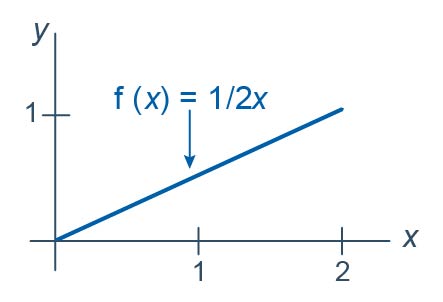
Let \(Y_1<Y_2<Y_3<Y_4<Y_5<Y_6\) be the order statistics associated with \(n=6\) independent observations each from the distribution with probability density function:
\(f(x)=\dfrac{1}{2}x\)
for \(0<x<2\). What is the probability that the next-to-largest order statistic, that is, \(Y_5\), is less than 1? That is, what is \(P(Y_5<1)\)?
Answer
The key to finding the desired probability is to recognize that the only way that the fifth order statistic, \(Y_5\), would be less than one is if at least 5 of the random variables \(X_1, X_2, X_3, X_4, X_5, \text{ and }X_6\) are less than one. For the sake of simplicity, let's suppose the first five observed values \(x_1, x_2, x_3, x_4, x_5\) are less than one, but the sixth \(x_6\) is not. In that case, the observed fifth-order statistic, \(y_5\), would be less than one:

The observed fifth order statistic, \(y_5\), would also be less than one if all six of the observed values \(x_1, x_2, x_3, x_4, x_5, x_6\) are less than one:

The observed fifth order statistic, \(y_5\), would not be less than one if the first four observed values \(x_1, x_2, x_3, x_4\) are less than one, but the fifth \(x_5\) and sixth \(x_6\) is not:

Again, the only way that the fifth order statistic, \(Y_5\), would be less than one is if 5 or 6... that is, at least 5... of the random variables \(X_1, X_2, X_3, X_4, X_5, \text{ and }X_6\) are less than one. For the sake of simplicity, we considered just the first five or six random variables, but in reality, any five or six random variables less than one would do. We just have to do some "choosing" to count the number of ways that we can get any five or six of the random variables to be less than one.
If you think about it, then, we have a binomial probability calculation here. If the event \(\{X_i<1\}\), \(i=1, 2, \cdots, 5\) is considered a "success," and we let \(Z\) = the number of successes in six mutually independent trials, then \(Z\) is a binomial random variable with \(n=6\) and \(p=0.25\):
\(P(X_i\le1)=\dfrac{1}{2}\int_{0}^{1}x dx=\dfrac{1}{2}\left[\dfrac{x^2}{2}\right]_{x=0}^{x=1}=\dfrac{1}{2}\left(\dfrac{1}{2}-0\right)=\dfrac{1}{4}\)
Finding the probability that the fifth order statistic, \(Y_5\), is less than one reduces to a binomial calculation then. That is:
\(P(Y_5<1)=P(Z=5)+P(Z=6)=\binom{6}{5}\left(\dfrac{1}{4} \right)^5\left(\dfrac{3}{4} \right)^1+\binom{6}{6}\left(\dfrac{1}{4} \right)^6\left(\dfrac{3}{4} \right)^0=0.0046\)
The fact that the calculated probability is so small should make sense in light of the given p.d.f. of \(X\). After all, each individual \(X_i\) has a greater chance of falling above, rather than below, one. For that reason, it would unusual to observe as many as five or six \(X\)'s less than one.
What is the cumulative distribution function \(G_5(y)\) of the fifth order statistic \(Y_5\)?
Answer
Recalling the definition of a cumulative distribution function, \(G_5(y)\) is defined to be the probability that the fifth order statistic \(Y_5\) is less than some value \(y\). That is:
\(G_5(y)=P(Y_5 < y)\)
Well, in our above work, we found the probability that the fifth order statistic \(Y_5\) is less than a specific value, namely 1. We just need to generalize our work there to allow for any value \(y\). Well, if the event \(\{X_i<y\}\), \(i=1, 2, \cdots, 5\) is considered a "success," and we let \(Z\) = the number of successes in six mutually independent trials, then \(Z\) is a binomial random variable with \(n=6\) and probability of success:
\(P(X_i\le y)=\dfrac{1}{2}\int_{0}^{y}x dx=\dfrac{1}{2}\left[\dfrac{x^2}{2}\right]_{x=0}^{x=y}=\dfrac{1}{2}\left(\dfrac{y^2}{2}-0\right)=\dfrac{y^2}{4}\)
Therefore, the cumulative distribution function \(G_5(y)\) of the fifth order statistic \(Y_5\) is:
\(G_5(y)=P(Y_5 < y)=P(Z=5)+P(Z=6)=\binom{6}{5}\left(\dfrac{y^2}{4}\right)^5\left(1-\dfrac{y^2}{4}\right)+\left(\dfrac{y^2}{4}\right)^6\)
for \(0<y<2\).
What is the probability density function \(g_5(y)\) of the fifth order statistic \(Y_5\)?
Answer
All we need to do to find the probability density function \(g_{5}(y)\) is to take the derivative of the distribution function \(G_5(y)\) with respect to \(y\). Doing so, we get:
\(g_5(y)=G_{5}^{'}(y)=\binom{6}{5}\left(\dfrac{y^2}{4}\right)^5\left(\dfrac{-2y}{4}\right)+\binom{6}{5}\left(1-\dfrac{y^2}{4}\right)5\left(\dfrac{y^2}{4}\right)^4\left(\dfrac{2y}{4}\right)+6\left(\dfrac{y^2}{4}\right)^5\left(\dfrac{2y}{4}\right)\)
Upon recognizing that:
\(\binom{6}{5}=6\) and \(\binom{6}{5}\times5=\dfrac{6!}{5!1!}\times5=\dfrac{6!}{4!1!}\)
we see that the middle term simplifies somewhat, and the first term is just the negative of the third term, therefore they cancel each other out:
\(g_{5}(y)=\left(\begin{array}{l}
6 \\
5
\end{array}\right)\color{red}\cancel {\color{black}\left(\frac{y^{2}}{4}\right)^{5}\left(\frac{-2 y}{4}\right)}\color{black}+\frac{6 !}{4 ! 1 !}\left(1-\frac{y^{2}}{4}\right)\left(\frac{y^{2}}{4}\right)^{4}\left(\frac{2 y}{4}\right)+\color{red}\cancel {\color{black}6\left(\frac{y^{2}}{4}\right)^{5}\left(\frac{2 y}{4}\right)}\)
Therefore, the probability density function of the fifth order statistic \(Y_5\) is:
\(g_5(y)=\dfrac{6!}{4!1!}\left(1-\dfrac{y^2}{4}\right)\left(\dfrac{y^2}{4}\right)^4\left(\dfrac{1}{2}y\right)\)
for \(0<y<2\). When we go on to generalize our work on the next page, it will benefit us to note that because the density function and distribution function of each \(X\) are:
\(f(x)=\dfrac{1}{2}x\) and \(F(x)=\dfrac{x^2}{4}\)
respectively, when \(0<x<2\), we can alternatively write the probability density function of the fifth order statistic \(Y_5\) as:
\(g_5(y)=\dfrac{6!}{4!1!}\left[F(y)\right]^4\left[1-F(y)\right]f(y)\)
Done!
Whew! Now, let's push on to the more general case of finding the probability density function of the \(r^{th}\) order statistic.
18.2 - The Probability Density Functions
18.2 - The Probability Density FunctionsOur work on the previous page with finding the probability density function of a specific order statistic, namely the fifth one of a certain set of six random variables, should help us here when we work on finding the probability density function of any old order statistic, that is, the \(r^{th}\) one.
Let \(Y_1<Y_2<\cdots, Y_n\) be the order statistics of n independent observations from a continuous distribution with cumulative distribution function \(F(x)\) and probability density function:
\( f(x)=F'(x) \)
where \(0<F(x)<1\) over the support \(a<x<b\). Then, the probability density function of the \(r^{th}\) order statistic is:
\(g_r(y)=\dfrac{n!}{(r-1)!(n-r)!}\left[F(y)\right]^{r-1}\left[1-F(y)\right]^{n-r}f(y)\)
over the support \(a<y<b\).
Proof
We'll again follow the strategy of first finding the cumulative distribution function \(G_r(y)\) of the \(r^{th}\) order statistic, and then differentiating it with respect to \(y\) to get the probability density function \(g_r(y)\). Now, if the event \(\{X_i\le y\},\;i=1, 2, \cdots, r\) is considered a "success," and we let \(Z\) = the number of such successes in \(n\) mutually independent trials, then \(Z\) is a binomial random variable with \(n\) trials and probability of success:
\(F(y)=P(X_i \le y)\)
Now, the \(r^{th}\) order statistic \(Y_r\) is less than or equal to \(y\) only if r or more of the \(n\) observations \(x_1, x_2, \cdots, x_n\) are less than or equal to \(y\), which implies:
\(G_r(y)=P(Y_r \le y)=P(Z=r)+P(Z=r+1)+ ... + P(Z=n)\)
which can be written using summation notation as:
\(G_r(y)=\sum_{k=r}^{n} P(Z=k)\)
Now, we can replace \(P(Z=k)\) with the probability mass function of a binomial random variable with parameters \(n\) and \(p=F(y)\). Doing so, we get:
\(G_r(y)=\sum_{k=r}^{n}\binom{n}{k}\left[F(y)\right]^{k}\left[1-F(y)\right]^{n-k}\)
Rewriting that slightly by pulling the \(n^{th}\) term out of the summation notation, we get:
\(G_r(y)=\sum_{k=r}^{n-1}\binom{n}{k}\left[F(y)\right]^{k}\left[1-F(y)\right]^{n-k}+\left[F(y)\right]^{n}\)
Now, it's just a matter of taking the derivative of \(G_r(y)\) with respect to \(y\). Using the product rule in conjunction with the chain rule on the terms in the summation, and the power rule in conjunction with the chain rule, we get:
\(g_r(y)=\sum_{k=r}^{n-1}{n\choose k}(k)[F(y)]^{k-1}f(y)[1-F(y)]^{n-k}\\ +\sum_{k=r}^{n-1}[F(y)]^k(n-k)[1-F(y)]^{n-k-1}(-f(y))\\+n[F(y)]^{n-1}f(y) \) (**)
Now, it's just a matter of recognizing that:
\(\left(\begin{array}{l}
n \\
k
\end{array}\right) k=\frac{n !}{\color{blue}\underbrace{\color{black}k !}_{\underset{\text{}}{{\color{blue}\color{red}\cancel {\color{blue}k}\color{blue}(k-1)!}}}\color{black}(n-k) !} \times \color{red}\cancel {\color{black}k}\color{black}=\frac{n !}{(k-1) !(n-k) !}\)
and
\(\left(\begin{array}{l}
n \\
k
\end{array}\right)(n-k)=\frac{n !}{k !\color{blue}\underbrace{\color{black}(n-k) !}_{\underset{\text{}}{{\color{blue}\color{red}\cancel {\color{blue}(n-k)}\color{blue}(n- k -1)!}}}\color{black}} \times \color{red}\cancel {\color{black}(n-k)}\color{black}=\frac{n !}{k !(n-k-1) !}\)
Once we do that, we see that the p.d.f. of the \(r^{th}\) order statistic \(Y_r\) is just the first term in the summation in \(g_r(y)\). That is:
\(g_r(y)=\dfrac{n!}{(r-1)!(n-r)!}\left[F(y)\right]^{r-1}\left[1-F(y)\right]^{n-r}f(y)\)
for \(a<y<b\). As was to be proved! Simple enough! Well, okay, that's a little unfair to say it's simple, as it's not all that obvious, is it? For homework, you'll be asked to write out, for the case when \(n=6\) and r = 3, the terms in the starred equation (**). In doing so, you should see that for all but the first of the positive terms in the starred equation, there is a corresponding negative term, so that everything but the first term cancels out. After you get a chance to work through that exercise, then perhaps it would be fair to say simple enough!
Example 18-2 (continued)
Let \(Y_1<Y_2<Y_3<Y_4<Y_5<Y_6\) be the order statistics associated with \(n=6\) independent observations each from the distribution with probability density function:
\(f(x)=\dfrac{1}{2}x \)
for \(0<x<2\). What is the probability density function of the first, fourth, and sixth order statistics?
Solution
When we worked with this example on the previous page, we showed that the cumulative distribution function of \(X\) is:
\(F(x)=\dfrac{x^2}{4} \)
for \(0<x<2\). Therefore, applying the above theorem with \(n=6\) and \(r=1\), the p.d.f. of \(Y_1\) is:
\(g_1(y)=\dfrac{6!}{0!(6-1)!}\left[\dfrac{y^2}{4}\right]^{1-1}\left[1-\dfrac{y^2}{4}\right]^{6-1}\left(\dfrac{1}{2}y\right)\)
for \(0<y<2\), which can be simplified to:
\(g_1(y)=3y\left(1-\dfrac{y^2}{4}\right)^{5}\)
Applying the theorem with \(n=6\) and \(r=4\), the p.d.f. of \(Y_4\) is:
\(g_4(y)=\dfrac{6!}{3!(6-4)!}\left[\dfrac{y^2}{4}\right]^{4-1}\left[1-\dfrac{y^2}{4}\right]^{6-4}\left(\dfrac{1}{2}y\right)\)
for \(0<y<2\), which can be simplified to:
\(g_4(y)=\dfrac{15}{32}y^7\left(1-\dfrac{y^2}{4}\right)^{2}\)
Applying the theorem with \(n=6\) and \(r=6\), the p.d.f. of \(Y_6\) is:
\(g_6(y)=\dfrac{6!}{5!(6-6)!}\left[\dfrac{y^2}{4}\right]^{6-1}\left[1-\dfrac{y^2}{4}\right]^{6-6}\left(\dfrac{1}{2}y\right)\)
for \(0<y<2\), which can be simplified to:
\(g_6(y)=\dfrac{3}{1024}y^{11}\)
Fortunately, when we graph the three functions on one plot:
we see something that makes intuitive sense, namely that as we increase the number of the order statistic, the p.d.f. "moves to the right" on the support interval.
18.3 - Sample Percentiles
18.3 - Sample PercentilesIt can be shown, as the authors of our textbook illustrate, that the order statistics \(Y_1<Y_2<\cdots<Y_n\) partition the support of \(X\) into \(n+1\) parts and thereby create \(n+1\) areas under \(f(x)\) and above the \(x\)-axis, with each of the \(n+1\) areas equaling, on average, \( \dfrac{1}{n+1} \):
Now, if we recall that the (100p)th percentile \(\pi_p\) is such that the area under \(f(x)\) to the left of \(\pi_p\) is \(p\), then the above plot suggests that we should let \(Y_r\) serve as an estimator of \(\pi_p\), where \( p = \dfrac{r}{n+1}\):
It's for this reason that we use the following formal definition of the sample percentile.
- (100p)th percentile of the sample
- The (100p)th percentile of the sample is defined to be \(Y_r\), the \(r^{th}\) order statistic, where \(r=(n+1)p\). For cases in which \((n+1)p\) is not an integer, we use a weighted average of the two adjacent order statistics \(Y_r\) and \(Y_{r+1}\).
Let's try this definition out an example.
Example 18-3

A report from the Texas Transportation Institute on Congestion Reduction Strategies highlighted the extra travel time (due to traffic congestion) for commute travel per traveler per year in hours for 13 different large urban areas in the United States:
| Urban Area | Extra Hours per Traveler Per Year |
|---|---|
| Philadelphia | 40 |
| Miami | 48 |
| Phoenix | 49 |
| New York | 50 |
| Boston | 53 |
| Detroit | 54 |
| Chicago | 55 |
| Dallas-Fort Worth | 61 |
| Atlanta | 64 |
| Houston | 65 |
| Washington, DC | 66 |
| San Fransisco | 75 |
| Los Angeles | 98 |
Find the first quartile, the 40th percentile, and the median of the sample of \(n=13\) extra travel times.
Answer
Because \(r=(13+1)(0.25)=3.5\), the first quartile, alternatively known as the 25th percentile, is:
\(\tilde{q}_1 =y_3+0.5(y_4-y_3) = 0.5y_3+0.5y_4=0.5(49)+0.5(50)=49.5\)
Because \(r=(13+1)(0.4)=5.6\), the 40th percentile is:
\(\tilde{\pi}_{0.40} = y_5 + 0.6(y_6-y_5) =0.4y_5 + 0.6y_6 =0.4(53)+0.6(54)=53.6\)
Because \(r=(13+1)(0.5)=7\), the median is:
\(\tilde{m} =y_7 = 55\)
Lesson 19: Distribution-Free Confidence Intervals for Percentiles
Lesson 19: Distribution-Free Confidence Intervals for PercentilesOverview
In the previous lesson, we learned how to calculate a sample percentile as a point estimate of a population (or distribution) percentile. Just as it is a good idea to calculate confidence intervals for other population parameters, such as means and variances, it would be a good idea to learn how to calculate a confidence interval for percentiles of a population. That's what we'll work on doing in this lesson. As the title of the lesson suggests, we won't make any assumptions about the distribution of the data, that is, other than it being continuous.
Objectives
- To learn how to calculate a confidence interval for a median using order statistics.
- To learn how to calculate a confidence interval for any population percentile using order statistics.
19.1 - For A Median
19.1 - For A MedianThe Method
As is generally the case, let's motivate the method for calculating a confidence interval for a population median \(m\) by way of a concrete example. Suppose \(Y_1<Y_2<Y_3<Y_4<Y_5\) are the order statistics of a random sample of size \(n=5\) from a continuous distribution. Our work from the previous lesson tells us that \(Y_3\) serves as a good point estimator of the median \(m\). Let's see what we can come up with for a confidence interval given we have these order statistics at our disposal. Well, suppose we suggested that the interval constrained by the first and fifth order statistics, that is, \((Y_1, Y_5)\) would serve as a good interval. How confident can we be that the interval \(Y_1, Y_5)\) would contain the unknown population median \(m\)? To answer that question, we simply need to calculate the following probability:
\(P(Y_1<m<Y_5)\)
Calculating the probability reduces to a simple binomial calculation once we figure out all the ways in which the population median \(m\) is sandwiched between \(Y_1\) and \(Y_5\). Well, the population median m is sandwiched between \(Y_1\) and \(Y_5\), if the first order statistic is the only order statistic less than the median \(m\):
The population median \(m\) is sandwiched between \(Y_1\) and \(Y_5\), if the first two order statistics are the only order statistics less than the median \(m\):
The population median \(m\) is sandwiched between \(Y_1\) and \(Y_5\), if the first three order statistics are less than the median \(m\), and the fourth and fifth order statistics are greater than \(m\):
And, the population median \(m\) is sandwiched between \(Y_1\) and \(Y_5\), if the fifth order statistic is the only order statistic greater than the median \(m\):
This means that in order to calculate the probability \(P(Y_1<m<Y_5)\), we need to calculate the probability of each of the above events. Now, if we let \(W\) denote the number of \(X_i<m\), then \(W\) is a binomial random variable with \(n\) mutually independent trials and probability of success \(p=P(X_i<m)=0.5\). And, reviewing the events as depicted above, the desired probability is calculated as:
\(P(Y_1<m<Y_5)=P(W=1)+P(W=2)+P(W=3)+P(W=4)\)
The binomial p.m.f. (or, alternatively, the binomial table) makes the calculation straightforward:
\(P(Y_1<m<Y_5)=\sum_{k=1}^{4}P(W=k)=\sum_{k=1}^{4}\binom{5}{k}(0.5)^k(0.5)^{5-k}=0.9376 \)
So, the probability that the random interval \((Y_1, Y_5)\) contains the median \(m\) is 0.9376. We aren't always so lucky with arriving at a decent confidence coefficient on our first try. Sometimes we have to try again aiming to get a confidence coefficient that it as least 90%, but as close to 95% as possible. In this case, the confidence coefficient for the interval \((Y_2, Y_4)\) is:
\(P(Y_2<m<Y_4)=\sum_{k=2}^{3}P(W=k)=\sum_{k=2}^{3}\binom{5}{k}(0.5)^k(0.5)^{5-k}=0.6250 \)
Clearly, we would be better served to stick with the interval \((Y_1, Y_5)\) in this case. Let's take a look at an example.
Example 19-1

An ecology laboratory studied tree dispersion patterns for the sugar maple whose seeds are dispersed by the wind. In a 50-meter by 50-meter plot, the laboratory researchers measured distances between like trees yielding the following distances, in meters and in increasing order, for 19 sugar maple trees:
2.10 2.35 2.35 3.10 3.10 3.15 3.90 3.90 4.00 4.80
5.00 5.00 5.15 5.35 5.50 6.00 6.00 6.25 6.45
Find a reasonable confidence interval for the median.
Answer
Because there are \(n=19\) data points, \(y_{10}=4.80\) serves as a good point estimator for the population median m. Let's go up and down a few spots from there to consider:
\((y_6, y_{14})=(3.15, 5.35)\)
as a possible confidence interval for \(m\). The confidence coefficient associated with the interval \((Y_6, Y_{14})\) is calculated using a binomial table with \(n=19\) and \(p=0.5\):
\(P(Y_6<m<Y_{14})=P(6\le W \le 13)=P(W \le 13) -P(W \le 5)=0.9682-0.0318=0.9364 \)
We can therefore be 93.64% confident that the population median falls in the interval (3.15, 5.35).
Could we do any better? Well, if we were to use the narrower interval \((y_7, y_{13})=(3.90, 5.15)\) instead, its confidence coefficient is not quite as good:
\(P(Y_7<m<Y_{13})=P(7\le W \le 12)=P(W \le 12) -P(W \le 6)=0.9165-0.0835=0.8330 \)
Or, if we were to use the wider interval \((y_5, y_{15})=(3.10, 5.50)\) instead, its confidence coefficient is perhaps a bit too high:
\(P(Y_5<m<Y_{15})=P(5\le W \le 14)=P(W \le 14) -P(W \le 4)=0.9904-0.0096=0.9808 \)
In general, we should aim to get a confidence coefficient at least 90%, but as close to 95% as possible. And, we shouldn't really "shop around" for an interval after we've collected the data. We should decide in advance which confidence interval we are going to use, and commit to use it even after the data have been collected.
A Helpful Table
Yeehaw! The authors of your textbook did a very kind thing for us by calculating the confidence coefficients for confidence intervals for the median \(m\) for various sample sizes \(n\). The resulting confidence coefficients are reported in the following table (or you can look in your text book if you don't want to use a magnifying glass to see this one):
The reading of the table is pretty straightforward. For example, if we have a sample of size \(n=12\), the table tells us we can be 96.14% confident that the population median falls in the interval constrained by the third and tenth order statistic, that is, in the interval \((Y_3, Y_{10})\). And, if we have a sample of size \(n=18\), the table tells us we can be 96.92% confident that the population median falls in the interval constrained by the fifth and fourteenth order statistic, that is, in the interval \((Y_5, Y_{14})\).
Normal Approximations of the Confidence Coefficients
All of our confidence coefficient calculations have involved binomial probabilities. It stands to reason, then, that if our sample size \(n\) is larger than 20, say, we could use the normal approximation to the binomial distribution. In our case, \(W\), the number of \(X_i<m\), follows a binomial distribution with mean and variance:
\(\mu=np=0.5n\) and \(\sigma^2=np(1-p)=0.5(1-0.5)n=0.25n\)
respectively. Therefore:
\(Z=\frac{W-0.5n}{\sqrt{0.25n}} \)
follows, at least approximately, the standard normal \(N(0,1)\) distribution.
Example 19-2

A sample of 26 offshore oil workers took part in a simulated escape exercise, resulting in the following data on time (in seconds) to complete the escape:
325 325 334 339 356 356 359 359 363
364 364 366 369 370 373 373 374 375
389 392 393 394 397 402 403 424
Use the normal approximation to the binomial to find the approximate confidence coefficient associated with the \((Y_8, Y_{18})\) confidence interval for the median \(m\). (The data are from the journal article "Oxygen Consumption and Ventilation During Escape from an Offshore Platform," Ergonomics 1997: 281-292.)
Answer
In this case, the mean and variance are:
\(\mu=np=0.5(26)=13\) and \(\sigma^2=np(1-p)=0.5(1-0.5)n=0.25(26)=6.5\)
respectively. Therefore, the approximate confidence coefficient for the interval \((Y_8, Y_{18})\) is:
\(P(Y_8<m<Y_{18})=P(8 \le W \le 17)=P\left(\frac{7.5-13}{\sqrt{6.5}} < Z < \frac{17.5-13}{\sqrt{6.5}} \right)\)
which can be simplified to:
\(P(Y_8<m<Y_{18})=P(-2.16 \le Z \le 1.77)=0.9616 - 0.0154 = 0.9462\)
We can be approximately 94.6% confident that the median time of all escapes is between 359 and 375 seconds.
19.2 - For Any Percentile
19.2 - For Any PercentileThe method that we learned for finding a confidence interval for the median of a continuous distribution can be easily extended so that we can find a confidence interval for any percentile \(\pi_p\). The only thing we have to change is the probability of a success, that is, that \(X_i\) is less than \(\pi_p\):
\(p=P(X_i < \pi_p)\)
Then, the exact confidence coefficient is calculated just as before using the binomial distribution with parameters \(n\) and \(p\):
\(1-\alpha=P(Y_i < \pi_p < Y_j)=\sum_{k=i}^{j-1}\binom{n}{k}p^k(1-p)^{n-k}\)
And, for large samples of size \(n\ge 20\), say, an approximate confidence coefficient is calculated using the normal approximation to the binomial by way of the standard normal random variable:
\(Z=\dfrac{W-np}{\sqrt{np(1-p)}}\)
Once the sample is observed and the order statistics determined, then the known interval \((y_i, y_j)\) serves as a \(100(1-\alpha)\%\) confidence interval for the unknown population percentile \(\pi_p\). Let's revisit an example from the previous page.
Example 19-2 (continued)

A sample of 26 offshore oil workers took part in a simulated escape exercise, resulting in the following data on time (in seconds) to complete the escape:
325 325 334 339 356 356 359 359 363
364 364 366 369 370 373 373 374 375
389 392 393 394 397 402 403 424
Find a confidence interval for the 75th percentile, and calculate its confidence coefficient. (The data are from the journal article "Oxygen Consumption and Ventilation During Escape from an Offshore Platform," Ergonomics 1997: 281-292.)
Answer
Since \((0.75)(26+1)=20.25\), the weighted average of the 20th and 21st order statistic:
\(\tilde{\pi}_{0.75}=y_{20}+0.25(y_{21}-y_{20})=0.75y_{20}+0.25y_{21}=0.75(392)+0.25(393)=392.25\)
serves as a good point estimate of \(\pi_{0.75}\). To find a confidence interval for \(\pi_{0.75}\), let's move up and down a few order statistics from \(y_{20}\) to, say, \(y_{16}\) and \(y_{24}\). In that case, our interval is \((y_{16}, y_{24}=(373, 402)\) with an exact confidence coefficient calculated using a binomial distribution with n = 26 and p = 0.75 as:
\(P(Y_{16}<m<Y_{24})=P(16 \le W \le 23)=P(W \le 23)-P(W \le 15)=0.9742-0.0401=0.9341\)
We can be 93.4% confident that the 75th percentile of all escape times is between 373 and 402 seconds.
Because \(n=26\) here, we could have alternatively used the normal approximation to the binomial. In this case, the mean and variance are:
\(\mu=np=0.75(26)=19.5\) and \(\sigma^2 =np(1-p)=26(0.75)(1-0.75)=4.875\)
respectively. Therefore, the approximate confidence coefficient for the interval \((y_{16}, y_{24})\) is:
\(P(Y_{16}<m<Y_{24})=P(16 \le W \le 23)=P\left(\dfrac{15.5-19.5}{\sqrt{4.875}} < Z < \dfrac{23.5-19.5}{\sqrt{4.875}} \right)\)
which can be simplified to:
\(P(Y_{16}<m<Y_{24})=P(-1.81 \le Z \le 1.81)=0.9649-0.0359=0.929\)
As you can see, the normal approximation does quite well, as the approximate probability is 0.929 compared to the exact probability of 0.934.
Lesson 20: The Wilcoxon Tests
Lesson 20: The Wilcoxon TestsOverview
Most of the hypothesis testing procedures we have investigated so far depend on some assumption about the underlying distribution of the data, the normality of the data, for example. Distribution-free methods, while not completely "assumption-less" relax some of those distributional assumptions. In this lesson, we'll investigate three such hypothesis tests:
- the sign test for a median
- the signed rank test for a median
- the Wilcoxon test for testing the equality of two distributions
In each case, the assumptions made are much less stringent than those made when we learned how to conduct hypothesis tests about population parameters, such as the mean \(\mu\) and proportion p.
20.1 - The Sign Test for a Median
20.1 - The Sign Test for a MedianRecall that for a continuous random variable X, the median is the value m such that 50% of the time X lies below m and 50% of the time X lies above m, such as illustrated in this example here:
Throughout our discussion, and as the above illustration suggests, we'll assume that our random variable X is a continuous random variable with unknown median m. Upon taking a random sample \(X_1 , X_2 , \dots , X_n\), we'll be interested in testing whether the median m takes on a particular value \(m_0\). That is, we'll be interested in testing the null hypothesis:
\(H_0 \colon m = m_0 \)
against any of the possible alternative hypotheses:
\(H_A \colon m > m_0\) or \(H_A \colon m < m_0\) or \(H_A \colon m \ne m_0\)
Let's start by considering the quantity \(X_i - m_0\) for \(i = 1, 2, \dots , n\). If the null hypothesis is true, that is, \(m = m_0\), then we should expect about half of the \(x_i - m_0\) quantities obtained to be positive and half to be negative:
If instead, \(m > m_0\) , then we should expect more than half of the \(x_i - m_0\) quantities obtained to be positive and fewer than half to be negative:
Or, if instead, \(m < m_0\) , then we should expect fewer than half of the \(x_i - m_0\) quantities obtained to be positive and more than half to be negative:
This analysis of \(x_i - m_0\) under the three situations \(m = m_0\), \(m > m_0\) , and \(m < m_0\) suggests then that a reasonable test for testing the value of a median m should depend on \(X_i - m_0\) . That's exactly what the sign test for a median does. This is what we'll do:
- Calculate \(X_i - m_0\) for \(i = 1, 2, \dots , n\).
- Define N− = the number of negative signs obtained upon calculating \(X_i - m_0\) for \(i = 1, 2, \dots , n\).
- Define N+ = the number of positive signs obtained upon calculating \(X_i - m_0\) for \(i = 1, 2, \dots , n\).
Then, if the null hypothesis is true, that is, \(m = m_0\), then N− and N+ both follow a binomial distribution with parameters n and p = 1/2. That is:
\(N-\sim b\left(n, \frac{1}{2}\right)\) and \(N+\sim b\left(n, \frac{1}{2}\right)\)
Now, suppose we are interested in testing the null hypothesis \(H_0 \colon m = m_0\) against the alternative hypothesis \(H_A \colon m > m_0\). Then, if the alternative hypothesis were true, we should expect \(X_i - m_0\) to yield more positive (+) signs than would be expected if the null hypothesis were true:
In that case, we should reject the null hypothesis if n−, the observed number of negative signs, is too small, or alternatively, if the P-value as defined by:
\(P = P(N - \le n-)\)
is small, that is, less than or equal to \(\alpha\).
And, suppose we are interested in testing the null hypothesis \(H_0 \colon m = m_0\) against the alternative hypothesis \(H_A \colon m < m_0\). Then, if the alternative hypothesis were true, we should expect \(X_i - m_0\) to yield more negative (−) signs than would be expected if the null hypothesis were true:
In that case, we should reject the null hypothesis if n+, the observed number of positive signs, is too small, or alternatively, if the P-value as defined by:
\(P = P(N+ \le n+)\)
is small, that is, less than or equal to \(\alpha\).
Finally, if we are interested in testing the null hypothesis \(H_0 \colon m = m_0\) against the alternative hypothesis \(H_A \colon m \neq m_0\), it makes sense that we should reject the null hypothesis if we have too few negative signs or too few positive signs. Formally, we reject if \(n_{min}\), which is defined as the smaller of n− and n+, is too small. Alternatively, we reject if the P-value as defined by:
\(P = 2 \times P(N_{min} \le min(n-, n+))\)
is small, that is, less than or equal to \(\alpha\). Let's take a look at an example.
Example 20-1

Recent studies of the private practices of physicians who saw no Medicaid patients suggested that the median length of each patient visit was 22 minutes. It is believed that the median visit length in practices with a large Medicaid load is shorter than 22 minutes. A random sample of 20 visits in practices with a large Medicaid load yielded, in order, the following visit lengths:
9.4 13.4 15.6 16.2 16.4 16.8 18.1 18.7 18.9 19.1
 19.3 20.1 20.4 21.6 21.9 23.4 23.5 24.8 24.9 26.8
Based on these data, is there sufficient evidence to conclude that the median visit length in practices with a large Medicaid load is shorter than 22 minutes?
Answer
We are interested in testing the null hypothesis \(H_0 \colon m = 22\) against the alternative hypothesis \(H_A \colon m < 22\). To do so, we first calculate \(x_i − 22\), for \(i = 1, 2, \dots, 20\). Letting Minitab do the 20 subtractions for us, we get:
We can readily see that \(n+\), the observed number of positive signs, is 5. Therefore, we need to calculate how likely it would be to observe as few as 5 positive signs if the null hypothesis were true. Doing so, we get a P-value of 0.0207:
which is, of course, smaller than \(\alpha = 0.05\). The P-value tells us that it is not likely that we would observe so few positive signs if the null hypothesis were true. Therefore, we reject the null hypothesis in favor of the alternative hypothesis. There is sufficient evidence, at the 0.05 level, to conclude that the median visit length in practices with a large Medicaid load is shorter than 22 minutes.
Incidentally, we can use Minitab to conduct the sign test for us by selecting, under the Stat menu, Nonparametrics and then 1-Sample Sign. Doing so, we get:
Let's take a look at an example that illustrates how the sign test can even be applied to a situation in which the data are paired.
Example 20-2
A study is done to determine the effects of removing a renal blockage in patients whose renal function is impaired because of advanced metatstatic malignancy of nonurologic cause. The arterial blood pressure of a random sample of 10 patients is measured before and after surgery for treatment of the blockage yielded the following data:
Based on the sign test, can we conclude that the surgery tends to lower arterial blood pressure?
Answer
We are interested in testing the null hypothesis \(H_0 \colon m_D = m_{B−A} = 0\) against the alternative hypothesis \(H_A \colon m_D = m_{B−A} > 0\). To do so, we just have to conduct a sign test while treating the differences as the data. If we look at the differences, we see that one of the differences is neither positive or negative, but rather zero. In this case, the standard procedure is to remove the observation that produces the zero, and reduce the number of observations by one. That is, we conduct the sign test using n = 9 rather than n = 10.
Now, n−, the observed number of negative signs, is 1, which yields a P-value of 0.0195:
The P-value is less than 0.05. Therefore, we can reject the null hypothesis. There is sufficient evidence, at the 0.05 level, to conclude that the surgery tends to lower arterial blood pressure.
Again, we can use Minitab to conduct the sign test for us. Doing so, we get:
Let's close up our discussion of the sign test by taking a note of the following:
- The sign test was presented here as a test for the median \(H_0 \colon m = m_0\), but if we were to make the additional assumption that the distribution of X is symmetric, then the sign test is also a valid test for the mean \(H_0 \colon \mu = \mu_0\).
- A primary advantage of the sign test is that by using only the signs of the \(X_i - m_0\) quantities, the test completely obliterates the negative effect of outliers.
- A primary disadvantage of the sign test is that by using only the signs of the \(X_i - m_0\) quantities, we potentially lose useful information about the magnitudes of the \(X_i - m_0\) quantities. For example, which data have more evidence against the null hypothesis \(H_0 \colon m = m_0\)? (1, 1, −1) versus (5, 6, −1)? Or (1, 1, −1) versus (10000, 6, −1)?
That last point suggests that we might want to also consider a test that takes into account the magntitudes of the \(X_i - m_0\) quantities. That's exactly what the Wilcoxon signed rank test does. Let's go check it out.
20.2 - The Wilcoxon Signed Rank Test for a Median
20.2 - The Wilcoxon Signed Rank Test for a MedianDeveloped in 1945 by the statistician Frank Wilcoxon, the signed rank test was one of the first "nonparametric" procedures developed. It is considered a nonparametric procedure, because we make only two simple assumptions about the underlying distribution of the data, namely that:
- The random variable X is continuous
- The probablility density function of X is symmetric
Then, upon taking a random sample \(X_1 , X_2 , \dots , X_n\), we are interested in testing the null hypothesis:
\(H_0 : m=m_0\)
against any of the possible alternative hypotheses:
\(H_A : m > m_0\) or \(H_A : m < m_0\) or \(H_A : m \ne m_0\)
As we often do, let's motivate the procedure by way of example.
Example 20-3

Let \(X_i\) denote the length, in centimeters, of a randomly selected pygmy sunfish, \(i = 1, 2, \dots 10\). If we obtain the following data set:
5.0 3.9 5.2 5.5 2.8 6.1 6.4 2.6 1.7 4.3
can we conclude that the median length of pygmy sunfish differs significantly from 3.7 centimeters?
Answer
We are interested in testing the null hypothesis \(H_0: m = 3.7\) against the alternative hypothesis \(H_A: m ≠ 3.7\). In general, the Wilcoxon signed rank test procedure requires five steps. We'll introduce each of the steps as we apply them to the data in this example.
- Step 1
In general, calculate \(X_i − m_0\) for \(i = 1, 2, \dots , n\). In this case, we have to calculate \(X_i − 3.7\) for \(i = 1, 2, \dots , 10\):
- Step 2
In general, calculate the absolute value of \(X_i − m_0\), that is, \(|X_i − m_0|\) for \(i = 1, 2, \dots , n\). In this case, we have to calculate \(|X_i − 3.7|\) for \(i = 1, 2, \dots , 10\):
- Step 3
Determine the rank \(R_i, i = 1, 2,\dots , n\) of the absolute values (in ascending order) according to their magnitude. In this case, the value of 0.2 is the smallest, so it gets rank 1. The value of 0.6 is the next smallest, so it gets rank 2. We continue ranking the data in this way until we have assigned a rank to each of the data values:
- Step 4
Determine the value of W, the Wilcoxon signed-rank test statistic:
\( W=\sum_{i=1}^{n}Z_i R_i\)
where \(Z_i\) is an indicator variable with \(Z_i = 0\) if \(X_i − m_0\) is negative and \(Z_i = 1\) if \(X_i − m_0\) is positive. That is, with \(Z_i\) defined as such, W is then the sum of the positive signed ranks. In this case, because the first observation yields a positive \(X_1 − 3.7\), namely 1.3, \(Z_1 = 1\). Because the fifth observation yields a negative \(X_5 − 3.7\), namely −0.9, \(Z_5 = 0\). Determining \(Z_i\) as such for \(i = 1, 2, \dots , 10\), we get:
And, therefore W equals 40:
\( W=(1)(5)+(1)(1)+ ... +(0)(-8)+(1)(2) =5+1+6+7+9+10+2=40\)
- Step 5
Determine if the observed value of W is extreme in light of the assumed value of the median under the null hypothesis. That is, calculate the P-value associated with W, and make a decision about whether to reject or not to reject. Whoa, nellie! We're going to have to take a break from this example before we can finish, as we first have to learn something about the distribution of W.
The Distribution of W
As is always the case, in order to find the distribution of the discrete random variable W, we need:
- To find the range of possible values of W, that is, we need to specify the support of W
- To determine the probability that W takes on each of the values in the support
Let's tackle the support of W first. Well, the smallest that \(W=\sum_{i=1}^{n}Z_i R_i\) could be is 0. That would happen if each observation \(X_i\) fell below the value of the median \(m_0\) specified in the null hypothesis, thereby causing \(Z_i = 0\), for \(i = 1, 2, \dots , n\):
The largest that \(W=\sum_{i=1}^{n}Z_i R_i\) could be is \(\dfrac{n(n+1)}{2}\). That would happen if each observation fell above the value of the median \(m_0\) specified in the null hypothesis, thereby causing \(z_i = 1\), for \(i = 1, 2, \dots , n\):
and therefore W reduces to the sum of the integers from 1 to n:
\(W=\sum_{i=1}^{n}Z_i R_i=\sum_{i=1}^{n}=\dfrac{n(n+1)}{2}\)
So, in summary, W is a discrete random variable whose support ranges between 0 and n(n+1)/2.
Now, if we have a small sample size n, such as we do in the above example, we could use the exact probability distribution of W to calculate the P-values for our hypothesis tests. Errr.... first we have to determine the exact probability distribution of W. Doing so is very doable. It just takes some thinking and perhaps a bit of tedious work. Let's make our discussion concrete by considering a very small sample size, n = 3, say. In that case, the possible values of W are the integers 0, 1, 2, 3, 4, 5, 6. Now, each of the three data points would be assigned a rank \(R_i\) of either 1, 2, or 3, and depending on whether the data point fell above or below the hypothesized median \(m_0\), each of the three possible ranks 1, 2, or 3 would remain either a positive signed rank or become a negative signed rank. In this case, because we are considering such a small sample size, we can easily enumerate each of the possible outcomes, as well as sum W of the positive ranks to see how each arrangement results in one of the possible values of W:
There we have it. We're just about done with finding the exact probability distribution of W when n = 3. All we have to do is recognize that under the null hypothesis, each of the above eight arrangements (columns) is equally likely. Therefore, we can use the classical approach to assigning the probabilities. That is:
- P(W = 0) = 1/8, because there is only one way that W = 0
- P(W = 1) = 1/8, because there is only one way that W = 1
- P(W = 2) = 1/8, because there is only one way that W = 2
- P(W = 3) = 2/8, because there are two ways that W = 3
- P(W = 4) = 1/8, because there is only one way that W = 4
- P(W = 5) = 1/8, because there is only one way that W = 5
- P(W = 6) = 1/8, because there is only one way that W = 6
And, just to make sure that we haven't made an error in our calculations, we can verify that the sum of the probabilities over the support 0, 1, ..., 6 is indeed 1/8 + 1/8 + ... + 1/8 = 1.
Hmmm. That was easy enough. Let's do the same thing for a sample size of n = 4. Well, in that case, the possible values of W are the integers 0, 1, 2, ..., 10. Now, each of the four data points would be assigned a rank \(R_i\) of either 1, 2, 3, or 4, and depending on whether the data point fell above or below the hypothesized median \(m_0\), each of the three possible ranks 1, 2, 3, or 4 would remain either a positive signed rank or become a negative signed rank. Again, because we are considering such a small sample size, we can easily enumerate each of the possible outcomes, as well as sum W of the positive ranks to see how each arrangement results in one of the possible values of W:
Again, under the null hypothesis, each of the above 16 arrangements is equally likely, so we can use the classical approach to assigning the probabilities:
- P(W = 0) = 1/16, because there is only one way that W = 0
- P(W = 1) = 1/16, because there is only one way that W = 1
- P(W = 2) = 1/16, because there is only one way that W = 2
- P(W = 3) = 2/16, because there are two ways that W = 3
- and so on...
- P(W = 9) = 1/16, because there is only one way that W = 9
- P(W = 10) = 1/16, because there is only one way that W = 10
Do you want to do the calculation for the case where n = 5? Here's what the enumeration of possible outcomes looks like:
After having worked through finding the exact probability distribution of W for the cases where n = 3, 4, and 5, we should be able to make some generalizations. First, note that, in general, there are \(2^n\) total number of ways to make signed rank sums, and therefore the probability that W takes on a particular value w is:
\(P(W=w)=f(w)=\dfrac{c(w)}{2^n}\)
where c(w) = the number of possible ways to assign a + or a − to the first n integers so that \(\sum_{i=1}^{n}Z_i R_i=w\).
Okay, now that we have the general idea of how to determine the exact probability distribution of W, we can breathe a sigh of relief when it comes to actually analyzing a set of data. That's because someone else has done the dirty work for us for sample sizes n = 3, 4, ..., 12, and published the relevant results in a statistical table of W. (Our textbook authors chose not to include such a table in our textbook.) By relevant, I mean the probabilities in the "tails" of the distribution of W. After all, that's what P-values generally are, that is, probabilities in the tails of the distribution under the null hypothesis.
As the table of W suggests, our determination of the probability distribution of W when n = 4 agrees with the results published in the table:
because both we and the table claim that:
\(P(W \le 0)=P(W \ge 10)=0.062\)
and:
\(P(W \le 1)=P(W =0)+P(W =1)=0.062+0.062=0.125\)
\(P(W \ge 9)=P(W =9)+P(W =10)=0.062+0.062=0.125\)
Okay, it should be pretty obvious that working with the exact distribution of W is going to be pretty limiting when it comes to large sample sizes. In that case, we do what we typically do when we have large sample sizes, namely use an approximate distribution of W.
When the null hypothesis is true, for large n:
\(W'={\sum_{i=1}^{n}Z_i R_i - \dfrac{n(n+1)}{4} \over \sqrt{\frac{n(n+1)(2n+1)}{24}}}\)
follows an approximate standard normal distribution N(0, 1).
Proof
Because the Central Limit Theorem is at work here, the approximate standard normal distribution part of the theorem is trivial. Our proof therefore reduces to showing that the mean and variance of W are:
\(E(W)=\dfrac{n(n+1)}{4}\) and \(Var(W)=\dfrac{n(n+1)(2n+1)}{24}\)
respectively. To find E(W) and Var(W), note that \(W=\sum_{i=1}^{n}Z_i R_i\) has the same distribution of \(U=\sum_{i=1}^{n}U_i\) where:
- \(U_i\) with probability ½
- \(U_i = i\) with probability ½
In case that claim was less than obvious, consider this intuitive, hand-waving kind of argument:
- W and U are both sums of a subset of the numbers 1, 2, ..., n
- Under symmetry, an equally likely chance of getting assigned either a + or a − is equivalent to having an equally likely chance of being included in the sum or not.
At any rate, we therefore have:
\(E(W)=E(U)=\sum_{i=1}^{n}E(U_i)=\sum_{i=1}^{n}\left[0\left(\dfrac{1}{2}\right)+i\left(\dfrac{1}{2}\right) \right]=\dfrac{1}{2}\sum_{i=1}^{n}i=\dfrac{1}{2}\times\frac{n(n+1)}{2}=\dfrac{n(n+1)}{4} \)
and:
\(Var(W) =Var(U)=\sum_{i=1}^{n}Var(U_i)\)
because the Ui's are independent under the null hypothesis. Now:
\(Var(U_i) = E(U_{i}^{2})-E(U_i)^2 = \left[0^2\left(\dfrac{1}{2}\right)+i^2\left(\dfrac{1}{2}\right) \right]-\left(\dfrac{i}{2}\right)^2 = \dfrac{i^2}{2}-\dfrac{i^2}{4} = \dfrac{i^2}{4}\)
and therefore:
\(Var(W)=\sum_{i=1}^{n}Var(U_i)=\sum_{i=1}^{n}\dfrac{i^2}{4}=\dfrac{1}{4}\sum_{i=1}^{n}i^2=\dfrac{1}{4}\times\dfrac{n(n+1)(2n+1)}{6} \)
Therefore, in summary, under the null hypothesis, we have that:
\(W'=\dfrac{\sum_{i=1}^{n}Z_i R_i - \dfrac{n(n+1)}{4}}{\sqrt{\frac{n(n+1)(2n+1)}{24}}} \)
follows an approximate standard normal distribution as was to be proved.
Let's return to our example now to complete our work.
Example 20-3 (continued)
Let \(X_i\) denote the length of a randomly selected pygmy sunfish, \(i = 1, 2, \dots 10\). If we obtain the following data set:
5.0 3.9 5.2 5.5 2.8 6.1 6.4 2.6 1.7 4.3
can we conclude that the median length of pygmy sunfish differs significantly from 3.7 centimeters?
Answer
Recall that we are interested in testing the null hypothesis \(H_0 \colon m = 3.7\) against the alternative hypothesis \(H_A \colon m ≠ 3.7\). The last time we worked on this example, we got as far as determining that W = 40 for the given data set. Now, we just have to use what we know about the distribution of W to complete our hypothesis test. Well, in this case, with n = 10, our sample size is fairly small so we can use the exact distribution of W. The upper and lower percentiles of the Wilcoxon signed rank statistic when n = 10 are:
Therefore, our P-value is 2 × 0.116 = 0.232. Because our P-value is large, we cannot reject the null hypothesis. There is insufficient evidence at the 0.05 level to conclude that the median length of pygmy sunfish differs significantly from 3.7 centimeters.
Notes
A couple of notes are worth mentioning before we take a look at another example:
- Our textbook authors define \(W=\sum_{i=1}^{n}R_i\) as the sum of all of the ranks, as opposed to just the sum of the positive ranks. That is perfectly fine, but not the most typical way of defining W.
- W is based on the ranks of the deviations from the hypothesized median \(m_0\), not on the deviations themselves. In the above example, W = 40 even if x7 = 6.4 or 10000 (now that's a pretty strange sunfish) because its rank would be unchanged. It is in this sense that W protects against the effect of outliers.
Now for that last example.
Example 20-4

The median age of the onset of diabetes is thought to be 45 years. The ages at onset of a random sample of 30 people with diabetes are:
35.5 44.5 39.8 33.3 51.4 51.3 30.5 48.9 42.1 40.3
46.8 38.0 40.1 36.8 39.3 65.4 42.6 42.8 59.8 52.4
26.2 60.9 45.6 27.1 47.3 36.6 55.6 45.1 52.2 43.5
Assuming the distribution of the age of the onset of diabetes is symmetric, is there evidence to conclude that the median age of the onset of diabetes differs significantly from 45 years?
Answer
We are interested in testing the null hypothesis \(H_0 \colon m = 45\) against the alternative hypothesis \(H_A \colon m ≠ 45\). We can use Minitab's calculator and statistical functions to do the dirty work for us:
Then, summing the last column, we get:

Because we have a large sample (n = 30), we can use the normal approximation to the distribution of W. In this case, our P-value is defined as two times the probability that W ≤ 200. Therefore, using a half-unit correction for continuity, our transformed signed rank statistic is:
\(W'=\dfrac{200.5 - \left(\frac{30(31)}{4}\right)}{\sqrt{\frac{30(31)(61)}{24}}}=-0.6581 \)
Therefore, upon using a normal probability calculator (or table), we get that our P-value is:
\(P \approx 2 \times P(W' < -0.66)=2(0.2546) \approx 0.51 \)
Because our P-value is large, we cannot reject the null hypothesis. There is insufficient evidence at the 0.05 level to conclude that the median age of the onset of diabetes differs significantly from 45 years.
By the way, we can even be lazier and let Minitab do all of the calculation work for us. Under the Stat menu, if we select Nonparametrics, and then 1-Sample Wilcoxon, we get:
20.3 - Tied Observations
20.3 - Tied ObservationsAll of our examples thus far have involved unique observations. That is, there were no tied observations. Dealing with ties is simple enough. If the absolute values of the differences from \(m_0\) of two or more observations are equal, each observation is assigned the average of the corresponding ranks. The change this causes in the distribution of W is not all that great.
Example 20-5

Dental researchers have developed a new material for preventing cavities, a plastic sealant that is applied to the chewing surfaces of teeth. To determine whether the sealant is effective, it was applied to half of the teeth of each of 12 school-aged children. After two years, the number of cavities in the sealant-coated teeth and in the uncoated teeth were counted, resulting in the following data:
Is there sufficient evidence to indicate that sealant-coated teeth are less prone to cavities than are untreated teeth? (From Wackerly, Mendenhall, & Scheaffer, seventh edition.)
Answer
Let X denote the number of cavities in the uncoated teeth, and Y denote the number of cavities in the coated teeth. Then, we're interested in analyzing the differences D = X−Y. Specifically, if m is the median of the differences D = X−Y, then we're interested in testing the null hypothesis \(H_0 \colon m = 0\) against the alternative hypothesis \(H_A \colon m > 0\). Analyzing the differences, we see that two of the differences are 0, and so we eliminate them from the analysis:
Assigning ranks to the remaining 10 data points, we see that we have two sets of tied observations. Because there are four 1s, we assign them the average of the ranks 1, 2, 3, and 4, that is, 2.5. Having used up the ranks 1, 2, 3, and 4, because 2 is the next set of tied observations, the three 2s are assigned the average of the ranks 5, 6, and 7, that is, 6. Having used up the ranks from 1 to 7, the remaining three unique observations get assigned the ranks 8, 9, and 10. When all is said and done, W, the sum of the positive ranks is:
W = 6 + 6 + 2.5 + 2.5 + 9 + 10 + 8 = 44
The statistical table for W:
tells us that the P-value is P(W ≥ 44) = 0.053. There is just barely not enough evidence, at the 0.05 level, to reject the null hypothesis. (I do imagine that a larger sample may have lead to a significant result.)
Alternatively, we could have completely ignored the condition of the data, that is, whether or not there were ties, and put the data into the black box of Minitab, getting:
We see that our analysis is consistent with the results from Minitab, namely 10 data points yield a Wilcoxon statistic of 44.0 and a P-value of 0.051 (round-off error).
Lesson 21: Run Test and Test for Randomness
Lesson 21: Run Test and Test for RandomnessOverview

In this lesson, we'll learn how to use what is called the Run Test to test whether the distribution functions F(x) and G(y) of two continuous random variables X and Y, respectively, are equal. That is, we'll use the Run Test to test the null hypothesis:
\(H_0 : F(z)=G(z)\)
against any of the typical alternatives. Note that other than the requirement that the random variables be continuous, no other conditions about the distributions must be met in order for the Run Test to be an appropriate test.
We'll close the lesson with seeing one particular application of the Run Test, namely, that of testing whether a series of observations are random (as opposed to showing some trend or some cycling.)
21.1 - The Run Test
21.1 - The Run TestLet's start from the beginning... it seems reasonable to think that before we can derive a Run Test, we better know what actually constitutes a run.
What is a run?
Let's suppose we have \(n_1\) observations of the random variable X, and \(n_2\) observations of the random variable Y. Suppose we combine the two sets of independent observations into one larger collection of \(n_1 + n_2\) observations, and then arrange the observations in increasing order of magnitude. If we label from which set each of the ordered observations originally came, we might observe something like this:
where x denotes an observation of the random variable X and y denotes an observation of the random variable Y. (We might observe this, for example, if the X values were 0.1, 0.4, 0.5, 0.6, 0.8, and 0.9, and the Y values were 0.2, 0.3, 0.7, 1.0, 1.1, and 1.2). That is, in this case, the smallest of all of the observations is an X value, the second smallest of all of the observations is a Y value, the third smallest of all of the observations is a Y value, the fourth smallest of all of the observations is an X value, and so on. Now, each group of successive values of X and Y is what we call a run. So, in this example, we have six runs. If we instead observed this ordered arrangement:
we would have three runs. And, if we instead observed this ordered arrangement:
we would have eight runs.
Why runs?
The next obvious question is in what way might knowing the number of runs be helpful in testing the null hypothesis of the equality of the distributions F(x) and G(y). Let's investigate that question by taking a look at a few examples. Let's start with the case in which the distributions are equal. In that case, we might observe something like this:
In this particular example, there are eight runs. As you can see, this kind of a picture suggests that when the distributions are equal, the number of runs will likely be large.
Now, let's take a look at one way in which the distribution functions could be unequal. One possibility is that one of the distribution functions is at least as great as the other distribution function at all points z. This situation might look something like this:
In this particular example, there are only two runs. This kind of a situation suggests that when one of the distribution functions is at least as great as the other distribution function, the number of runs will likely be small. Note that this is what the distribution functions might look like if the median of Y was greater than the median of X.
Here's another way in which the distribution functions could be unequal:
In this case, the medians of X and Y are nearly equal, but the variance of Y is much greater than the variance of X. In this particular example, there are only three runs. Again, in general, when we have this type of situation, we would expect the number of runs to be small.
The above three examples give a pretty clear indication that we're onto something with the idea of using runs to test the null hypothesis of the equality of two distribution functions. If the number of runs is smaller than expected, it seems we should reject the null hypothesis, because a small number of runs suggests that there are differences in either the location or the spread of the two distributions. Now, as is usually the case when conducting a hypothesis test, in order to quantify "smaller than expected," we're going to need to know something about the distribution of R, the number of runs.
What is the p.m.f. of R?
Let's let the random variable R denote the number of runs in the combined ordered sample containing \(n_1\) observations of X and \(n_2\) observations of Y. With possible values, such as 2, 3, and so on, R is clearly discrete. Now, if the null hypothesis is true, that is, the distribution functions are equal, all of the possible permutations of the X's and the Y's in the combined sample are equally likely. Therefore, we can use the classical approach to assigning the probability that R equals a particular value r. That is, to find the distribution of R, we can find:
for all of the possible values in the support of R. (Note that the support depends on the number of observations in the combined sample. We do know, however, that R must be at least 2.) As is usually the case, the denominator is the easy part. If we have \(n_1 + n_2\) positions:

in which we can choose to place the \(n_1\) observed x values, then the total number of ways of arranging the x's and y's is:
\(\binom{n_1+n_2}{n_1}\)
Note that once the x values are placed in their positions, the remaining \(n_2\) positions must contain the y values. We just as easily could place the y values first, and then the remaining \(n_1\) positions must contain the x values.
Now for the numerator. That's the messy part! Before we even begin to attempt to generalize a formula for the quantity in the numerator, it might be best to take a look at a concrete example.
Example 21-1

Suppose we have \(n_1 = 3\) observations of the random variable X and \(n_2 = 3\) observations of the random variable Y. What is the p.m.f. of R, the number of runs?
Answer
Put your seatbelt on. If not your seatbelt, then at least your bookkeeping hat. This is going to get a bit messy at times. So... let's start with the easy part first... the denominator! If we combine the two samples, we have a total of 3+3 = 6 observations to arrange. Therefore, there are:
\(\binom{3+3}{3}=\binom{6}{3}=\dfrac{6!}{3! 3!}=20\)
possible ways of arranging the x's and y's. Now, that's a small enough number that we can actually enumerate all 20 of the possible arrangements. Here they are:
Now, as the above table suggests, of the 20 possible arrangements, there are two ways of getting R = 2 runs. Therefore:
\(P(R=2)=\frac{2}{20}\)
And, of the 20 possible arrangements, there are four ways of getting R = 3 runs. Therefore:
\(P(R=3)=\frac{4}{20}\)
Piece of cake! What was all this talk about messy bookkeeping? With the snap of a finger, we can determine the entire p.m.f. of R:
Note that the probabilities add to 1. That's a good sign! But finding the specific p.m.f. of R was not the point of this example. We were going to use this example to try to learn something about finding the p.m.f. of R in general. The only reason why we were able to find this p.m.f. of R with such ease was because we could enumerate all 20 of the possible outcomes. What if we can't do that? That is, what if there were so many possible arrangements that it would be crazy to try to enumerate them all? Well, we would go way back to what we did in Stat 414... we would derive a general counting formula! That's what we're working towards here.
Let's take a look at a case in which r is even, \(r = 4\), say. If you think about it, the only way we can get four runs is if the \(n_1 = 3\) values of X are broken up into 2 runs, which can be done in either of two ways:
and the \(n_2 = 3\) values of Y are broken up into 2 runs, which can be done in either of two ways:
Now, it's just a matter of putting the 2 runs of X and the 2 runs of Y together to make a total of 4 runs in the sequence. Well, there are two ways of getting 2 runs of X and two ways of getting 2 runs of Y. Therefore, the multiplication rule tells us that we should expect there to be 2×2 = 4 ways of getting four runs when the samples are combined. There's just one problem with that calculation, namely that there are 2 ways of starting the sequence off. That is, we could start with an X run:
or we could start with a Y run:
So, the multiplication rule actually tells us that there are \(2 \time 2 \times 2 = 8\) ways of getting four runs when we have \(n_1 = 3\) values of X and \(n_2 = 3\) values of Y. And, we've just enumerated all eight of them!
Now, let's try to generalize the above process. We started by considering a case in which r was even, specifically, r = 4. Note that r is even implies that \(r = 2k\), for a positive integer k. (If \(r = 4\), for example, then \(k = 2\).) Now, the only way we can get \(r = 4\) runs is if the \(n_1 = 3\) values of X are broken up into \(k = 2\) runs and the \(n_2 = 3\) values of Y are broken up into k = 2 runs. We can form the k = 2 runs of the \(n_1 = 3\) values of X by inserting \(k−1 = 1\) divider into the \(n_1 − 1 = 2\) spaces between the X values:
When the divider is here:
we create these two runs:
And, when the divider is here:
we create these two runs:
Note that, in general, there are:
\(\binom{n_1-1}{k-1}\)
ways of inserting k−1 dividers into the \(n_1 − 1\) spaces between the X values, with no more than one divider per space.
Now, we can go through the exact same process for the Y values. It shouldn't be too hard to see that, in general, there are:
\(\binom{n_2-1}{k-1}\)
ways of inserting k−1 dividers into the \(n_2 − 1\) spaces between the Y values, with no more than one divider per space.
Now, if you go back and look, once we broke up the X values into k = 2 runs, and the Y values into k = 2 runs, the next thing we did was to put the two sets of two runs of X and two sets of two runs of Y together. The multiplication rule tells us that there are:
\(\binom{n_1-1}{k-1}\binom{n_2-1}{k-1}\)
ways of putting the two sets of runs together to form \(r = 2k\) runs beginning with a run of x's. And, the multiplication rule tells us that there are:
\(\binom{n_2-1}{k-1}\binom{n_1-1}{k-1}\)
ways of putting the two sets of runs together to form \(r = 2k\) runs beginning with a run of y's. Therefore, the total number of ways of getting \(r = 2k\) runs is:
\(\binom{n_1-1}{k-1}\binom{n_2-1}{k-1}+\binom{n_2-1}{k-1}\binom{n_1-1}{k-1}=2\binom{n_1-1}{k-1}\binom{n_2-1}{k-1}\)
And, therefore putting the numerator and the denominator together, we get:
\(P(R=2k)=\frac{2\binom{n_1-1}{k-1}\binom{n_2-1}{k-1}}{\binom{n_1+n_2}{n_1}}\)
when k is a positive integer.
Whew! Now, we've found the probability of getting r runs when r is even. What happens if r is odd? That is, what happens if \(r = 2k+1\) for a positive integer k? Well, let's consider the case in which \(r = 3\), and therefore \(k = 1\). If you think about it, there are two ways we can get three runs... either we need \(k+1 = 2\) runs of x's and k = 1 run of y's, such as:
and 
or we need \(k = 1\) run of x's and \(k+1 = 2\) runs of y's:
 and
and
Perhaps you can see where this is going? In general, we can form \(k+1\) runs of the \(n_1\) values of X by inserting k dividers into the \(n_1−1\) spaces between the X values, with no more than one divider per space, in:
\(\binom{n_1-1}{k}\)
ways. Similarly, we can form k runs of the \(n_2\) values of Y in:
\(\binom{n_2-1}{k-1}\)
ways. The two sets of runs can be placed together to form \(2k+1\) runs in:
\(\binom{n_1-1}{k}\binom{n_2-1}{k-1}\)
ways. Likewise, \(k+1\) runs of the \(n_2\) values of Y, and k runs of the \(n_1\) values of X can be placed together to form:
\(\binom{n_2-1}{k}\binom{n_1-1}{k-1}\)
sets of \(2k+1\) runs. Therefore, the total number of ways of getting \(r = 2k+1\) runs is:
\(\binom{n_1-1}{k}\binom{n_2-1}{k-1}+\binom{n_2-1}{k}\binom{n_1-1}{k-1}\)
And, therefore putting the numerator and the denominator together, we get:
\(P(R=2k+1)=\frac{\binom{n_1-1}{k}\binom{n_2-1}{k-1}+\binom{n_2-1}{k}\binom{n_1-1}{k-1}}{\binom{n_1+n_2}{n_1}} \)
Yikes! Let's put this example to rest!
Let's summarize what we've learned.
Summary. The probability that R, the number of runs, takes on a particular value r is:
\(P(R=2k)=\dfrac{2\binom{n_1-1}{k-1}\binom{n_2-1}{k-1}}{\binom{n_1+n_2}{n_1}}\)
if r is even, that is, if \(r = 2k\) for a positive integer k. The probability that R, the number of runs, takes on a particular value r is:
\(P(R=2k+1)=\dfrac{\binom{n_1-1}{k}\binom{n_2-1}{k-1}+\binom{n_2-1}{k}\binom{n_1-1}{k-1}}{\binom{n_1+n_2}{n_1}} \)
if r is odd, that is, if\(r = 2k + 1\) for a positive integer k.
Now, let's wrap up our development of the Run Test with an example.
Example 21-2

Let X and Y denote the times in hours per weeks that students in two different schools watch television. Let F(x) and G(y) denote the respective distributions. To test the null hypothesis:
\(H_0 : F(z) =G(z)\)
a random sample of eight students was selected from each school, yielding the following results:

What conclusion should we make about the equality of the two distribution functions?
Answer
The combined ordered sample, with the x values in blue and the y values in red, looks like this:
Counting, we see that there are 9 runs. We should reject the null hypothesis if the number of runs is smaller than expected. Therefore, the critical region should be of the form r ≤ c. In order to determine what we should set the value of c to be, we'll need to know something about the p.m.f. of R. We can use the formulas that we derived above to determine various probabilities. Well, with \(n_1 = 8 , n_2 = 8 , \text{ and } k = 1\), we have:
\(P(R=2)=\dfrac{2\binom{7}{0}\binom{7}{0}}{\binom{16}{8}}=\dfrac{2}{12,870}=0.00016\)
and:
\(P(R=3)=\dfrac{\binom{7}{1}\binom{7}{0}+\binom{7}{1}\binom{7}{0}}{\binom{16}{8}}=\dfrac{14}{12,870}=0.00109\)
(Note that Table I in the back of the textbook can be helpful in evaluating the value of the "binomial coefficients.") Now, with \(n_1 = 8 , n_2 = 8 , \text{ and } k = 2\), we have:
\(P(R=4)=\dfrac{2\binom{7}{1}\binom{7}{1}}{\binom{16}{8}}=\dfrac{98}{12,870}=0.00761\)
and:
\(P(R=5)=\dfrac{\binom{7}{2}\binom{7}{1}+\binom{7}{2}\binom{7}{1}}{\binom{16}{8}}=\dfrac{294}{12,870}=0.02284\)
And, with \(n_1 = 8 , n_2 = 8 , \text{ and } k = 3\), we have:
\(P(R=6)=\dfrac{2\binom{7}{2}\binom{7}{2}}{\binom{16}{8}}=\dfrac{882}{12,870}=0.06853\)
Let's stop to see what we have going for us so far. Well, so far we've learned that:
\(P(R \le 6)=0.00016+0.00109+0.00761+0.02284+0.06853=0.1002\)
Hmmm. That tells us that if we set c = 6, we'd have a 0.1002 probability of committing a Type I error. That seems reasonable! That is, let's decide to reject the null hypothesis of the equality of the two distribution functions if the number of observed runs \(r ≤ 6\). It's not... we observed 9 runs. Therefore, we fail to reject the null hypothesis at the 0.10 level. There is insufficient evidence at the 0.10 level to conclude that the distribution functions are not equal.
A Large-Sample Test
As our work in the previous example illustrates, conducting a single run test can be quite extensive in the calculation front. Is there an easier way? Fortunately, yes... that is, providing \(n_1\) and \(n_2\) are large. Typically, we consider the samples to be large if \(n_1\) is at least 10 and \(n_2\) is at least 10. If the samples are large, then the distribution of R can be approximated with a normally distributed random variable. That is, it can be shown that:
\(Z=\dfrac{R-\mu_R}{\sqrt{Var(R)}}\)
follows an approximate standard normal \(N(0, 1)\) distribution with mean:
\(\mu_R=E(R)=\dfrac{2n_1n_2}{n_1+n_2}+1 \)
and variance:
\( Var(R)=\dfrac{2n_1n_2(2n_1n_2-n_1-n_2)}{(n_1+n_2)^2(n_1+n_2-1)}\).
Because a small number of runs is evidence that the distribution functions are unequal, the critical region for testing the null hypothesis:
\(H_0 : F(z) = G(z)\)
is of the form \(z ≤ −z_{\alpha}\), where \(\alpha\) is the desired significance level. Let's take a look at an example.
Example 21-3

A charter bus line has 48-passenger buses and 38-passenger buses. With X and Y denoting the number of miles traveled per day for the 48-passenger and 38-passenger buses, respectively, the bus company is interested in testing the equality of the two distributions:
\(H_0 : F(z) = G(z)\)
The company observed the following data on a random sample of \(n_1 = 10\) buses holding 48 passengers and \(n_2 = 11\) buses holding 38 passengers:

Using the normal approximation to R, conduct the hypothesis test at the 0.05 level.
Answer
The combined ordered sample, with the x values in blue and the y values in red, looks like this:
Counting, we see that there are 9 runs. Using the normal approximation to R, with \(n_1 = 10\) and \(n_2 = 11\), we have:
\(\mu_R=\dfrac{2n_1n_2}{n_1+n_2}+1=\dfrac{2(10)(11)}{10+11}+1=11.476\)
and:
\( Var(R)=\dfrac{2n_1n_2(2n_1n_2-n_1-n_2)}{(n_1+n_2)^2(n_1+n_2-1)} =\dfrac{2(10)(11)[2(10)(11)-10-11]}{(10+11)^2(10+11-1)}=4.9637\)
Now, we observed r = 9 runs. Therefore, the approximate P-value, using a half-unit correction for continuity, is:
\(P \approx P\left[Z \le \dfrac{9.5-11.476}{\sqrt{4.9637}} \right]=P[Z \le -0.89]=0.187\)
We fail to reject the null hypothesis at the 0.05 level, because the P-value is greater than 0.05. There is insufficient evidence at the 0.05 level to conclude that the two distribution functions are unequal.
21.2 - Test for Randomness
21.2 - Test for RandomnessA common application of the run test is a test for randomness of observations. Because an interest in randomness of observations is quite often seen in a quality-control setting, that's the application that will be the focus of our attention. For example, suppose a quality control supervisor at a paint manufacturing company suspects that the weights of paint cans on the production line are not varying in a random way, as she would expect. Instead, she suspects that the weights are either trending upward or are varying in a cyclic fashion. Every ten minutes, she randomly samples a paint can from the production line, and determines the weights of the randomly selected can.
Let's let \(x_1, x_2, \dots , x_N\) denote the observed weights, where the subscripts designate the order in which the outcomes were obtained. (Note that the textbook uses the letter k here to denote the number of observations in the sample, an unfortunate choice, I think, because we've already taken k to mean something else in this lesson. At any rate, just to be different, and hopefully clearer, I'll use a capital letter N to denote the total number of observations in the sample.) For the sake of concreteness, let's suppose that N is even. If we calculate the median m of the observed weights, then by definition, the median divides the observed sample in half. That is, half of the weights will be less than the median, and half of the weights will be greater than the median. Now, suppose we replace each observation by L if it falls below the median, and by U if it falls above the median.
-
If we observe something like this:
U U U U L U L L L L
then the production process is showing a trend. In this case, we would not observe as many runs r as we would expect if the process were truly random. In this case, we would reject the null hypothesis of randomness, in favor of the alternative hypothesis of a trend effect, if \(r ≤ c\).
-
If we instead observed something like this:
U L U L U L U L U L
then the production process is showing some kind of cyclic event. In this case, we would observe more runs r than we would expect if the process were truly random. In this case, we would reject the null hypothesis of randomness, in favor of the alternative hypothesis of a cyclic effect, if \(r ≥ c\).
-
If we aren't sure in which way a process would deviate from randomness, then we should allow for the possibility of either a trend effect or a cyclic effect. In this case, we should reject the null hypothesis of randomness, in favor of the alternative hypothesis of either a trend effect or a cyclic effect, if \(r ≤ c\) or \(r ≥ c\).
Let's try this idea out on an example!
Example 21-4

A quality control chart has been maintained for the weights of paint cans taken from a conveyor belt at a fixed point in a production line. Sixteen (16) weights obtained today, in order of time, are as follows:
Use the run test, at approximately a 0.01 level, to determine whether the weights of the paint cans on the conveyor belt deviate from randomness.
Answer
With just a bit of ordering work (or using Minitab or some other statistical software), we can readily determine that the median weight of the sampled paint cans is 67.9. Labeling each observed weight with either a U if the observed weight is greater than the median (67.9), or an L if the observed weight is less than the median (67.9), we get:
Counting, we see that we observe 7 runs. Because there is no specific direction given in the possible deviation from randomness, we should test for both trend and cyclic effects. That is, we should reject the null hypothesis if we have either too few or too many runs. That is, our rejection region should be of the form:
\({r : r ≤ c \text{ or } r ≥ c}\)
Because we have a sample size of N = 16, we'll use the p.m.f. of R with \(n_1 = 8\) and \(n_2 = 8\). Now, using the formulas with k = 1 and k = 8, we get:
\[P(R=2)=\dfrac{2\binom{7}{0}\binom{7}{0}}{\binom{16}{8}}=\dfrac{2\binom{7}{7}\binom{7}{7}}{\binom{16}{8}} =P(R=16)=\dfrac{2}{12,870} \]
Using the formulas with k = 1 and k = 7, we get:
\[P(R=3)=\dfrac{\binom{7}{1}\binom{7}{0}+\binom{7}{1}\binom{7}{0}}{\binom{16}{8}}=\dfrac{\binom{7}{7}\binom{7}{6}+\binom{7}{7}\binom{7}{6}}{\binom{16}{8}}=P(R=15)=\dfrac{14}{12,870} \]
And, using the formulas with k = 2 and k = 7, we get:
\[P(R=4)=\dfrac{2\binom{7}{1}\binom{7}{1}}{\binom{16}{8}}=\dfrac{2\binom{7}{6}\binom{7}{6}}{\binom{16}{8}} =P(R=14)=\dfrac{98}{12,870} \]
Therefore, the critical region \({r : r ≤ 4 \text{ or } r ≥ 14}\) would yield a test at a significance level of:
\[\alpha = P(R \le 4)+P(R \ge 14)=\dfrac{2+14+98}{12,870}+\dfrac{2+14+98}{12,870}=\dfrac{228}{12,870}=0.018\]
The 7 runs we observed does not fall in our proposed rejection region. Therefore, we fail to reject at the 0.018 significance level. There is insufficient evidence at the 0.018 level to conclude that the process has deviated from randomness.
Notes
- In both the discussion and the example above, the sample size N was even. What happens if the sample size N is odd? Well, in that case, when we divide the sample up into those below (L) and those above (U) the median, the number of observations in the "upper half" and the "lower half" will differ by one. If that's the case, the standard protocol is to put the extra observation in the "upper half." In that case, \(n_2 = n_1 + 1\).
- If the median is equal to a value that is tied with other values, standard protocol again puts the tied values in the "upper half," and the test is performed with \(n_1\) and \(n_2\) being unequal.
Lesson 22: Kolmogorov-Smirnov Goodness-of-Fit Test
Lesson 22: Kolmogorov-Smirnov Goodness-of-Fit TestOverview

In this lesson, we'll learn how to conduct a test to see how well a hypothesized distribution function \(F(x)\) fits an empirical distribution function \(F_{n}(x)\). The "goodness-of-fit test" that we'll learn about was developed by two probabilists, Andrey Kolmogorov and Vladimir Smirnov, and hence the name of this lesson. In the process of learning about the test, we'll:
- learn a formal definition of an empirical distribution function
- justify, but not derive, the Kolmogorov-Smirnov test statistic
- try out the test on a few examples
- learn how to calculate a confidence band for a distribution function \(F(x)\)
22.1 - The Test
22.1 - The TestBefore we can work on developing a hypothesis test for testing whether an empirical distribution function \(F_n (x)\) fits a hypothesized distribution function \(F (x)\) we better have a good idea of just what is an empirical distribution function \(F_n (x)\). Therefore, let's start with formally defining it.
- Empirical distribution function
-
Given an observed random sample \(X_1 , X_2 , \dots , X_n\), an empirical distribution function \(F_n (x)\) is the fraction of sample observations less than or equal to the value x. More specifically, if \(y_1 < y_2 < \dots < y_n\) are the order statistics of the observed random sample, with no two observations being equal, then the empirical distribution function is defined as:
That is, for the case in which no two observations are equal, the empirical distribution function is a "step" function that jumps \(1/n\) in height at each observation \(x_k\). For the cases in which two (or more) observations are equal, that is, when there are \(n_k\) observations at \(x_k\), the empirical distribution function is a "step" function that jumps \(n_k/n\) in height at each observation \(x_k\). In either case, the empirical distribution function \(F_n(x)\) is the fraction of sample values that are equal to or less than x.
Such a formal definition is all well and good, but it would probably make even more sense if we took at a look at a simple example.
Example 22-1

A random sample of n = 8 people yields the following (ordered) counts of the number of times they swam in the past month:
0 1 2 2 4 6 6 7
Calculate the empirical distribution function \(F_n (x)\).
Answer
As reported, the data are ordered, therefore the order statistics are \(y_1 = 0, y_2 = 1, y_3 = 2, y_4 = 2, y_5 = 4, y_6 = 6, y_7 = 6\) and \(y_8 = 7\). Therefore, using the definition of the empirical distribution function, we have:
\(F_n(x)=0 \text{ for } x < 0\)
and:
\(F_n(x)=\frac{1}{8} \text{ for } 0 \le x < 1\) and \(F_n(x)=\frac{2}{8} \text{ for } 1 \le x < 2\)
Now, noting that there are two 2s, we need to jump 2/8 at x = 2:
\(F_n(x)=\frac{2}{8}+\frac{2}{8}=\frac{4}{8} \text{ for } 2 \le x < 4\)
Then:
\(F_n(x)=\frac{5}{8} \text{ for } 4 \le x < 6\)
Again, noting that there are two 6s, we need to jump 2/8 at x = 6:
\(F_n(x)=\frac{5}{8}+\frac{2}{8}=\frac{7}{8} \text{ for } 6 \le x < 7\)
And, finally:
\(F_n(x)=\frac{7}{8}+\frac{1}{8}=\frac{8}{8}=1 \text{ for } x \ge 7\)
Plotting the function, it should look something like this then:
Now, with that behind us, let's jump right in and state and justify (not prove!) the Kolmogorov-Smirnov statistic for testing whether an empirical distribution fits a hypothesized distribution well.
- Kolmogorov-Smirnov test statistic
-
\[D_n=sup_x\left[ |F_n(x)-F_0(x)| \right]\]
is used for testing the null hypothesis that the cumulative distribution function \(F (x)\) equals some hypothesized distribution function \(F_0 (x)\), that is, \(H_0 : F(x)=F_0(x)\), against all of the possible alternative hypotheses \(H_A : F(x) \ne F_0(x)\). That is, \(D_n\) is the least upper bound of all pointwise differences \(|F_n(x)-F_0(x)|\).
The bottom line is that the Kolmogorov-Smirnov statistic makes sense, because as the sample size n approaches infinity, the empirical distribution function \(F_n (x)\) converges, with probability 1 and uniformly in x, to the theoretical distribution function \(F (x)\). Therefore, if there is, at any point x, a large difference between the empirical distribution \(F_n (x)\) and the hypothesized distribution \(F_0 (x)\), it would suggest that the empirical distribution \(F_n (x)\) does not equal the hypothesized distribution \(F_0 (x)\). Therefore, we reject the null hypothesis:
\[H_0 : F(x)=F_0(x)\]
if \(D_n\) is too large.
Now, how do we know that \(F_n (x)\) converges, with probability 1 and uniformly in x, to the theoretical distribution function \(F (x)\)? Well, unfortunately, we don't have the tools in this course to officially prove it, but we can at least do a bit of a hand-waving argument.
Let \(X_1 , X_2 , \dots , X_n\) be a random sample of size n from a continuous distribution \(F (x)\). Then, if we consider a fixed x, then \(W= F_n (x)\) can be thought of as a random variable that takes on possible values \(0, 1/n , 2/n , \dots , 1\). Now:
- nW = 1, if and only if exactly 1 observation is less than or equal to x, and n−1 observations are greater than x
- nW = 2, if and only if exactly 2 observations are less than or equal to x, and n−2 observations are greater than x
- and in general...
- nW = k, if and only if exactly k observations are less than or equal to x, and n−k observations are greater than x
If we treat a success as an observation being less than or equal to x, then the probability of success is:
\(P(X_i ≤ x) = F(x)\)
Do you see where this is going? Well, because \(X_1 , X_2 , \dots , X_n\) are independent random variables, the random variable nW is a binomial random variable with n trials and probability of success p = F(x). Therefore:
\[ P\left(W = \frac{k}{n}\right) = P(nW=k) = \binom{n}{k}[F(x)]^k[1-F(x)]^{n-k}\]
And, the expected value and variance of nW are:
\(E(nW)=np=nF(x)\) and \(Var(nW)=np(1-p)=n[F(x)][1-F(x)]\)
respectively. Therefore, the expected value and variance of W are:
\(E(W)=n\frac{F(x)}{n}=F(x)\) and \(\displaystyle Var(W) =\frac{n[(F(x)][1-F(x)]}{n^2}=\frac{[(F(x)][1-F(x)]}{n}\)
We're very close now. We just now need to recognize that as n approaches infinity, the variance of W, that is, the variance of \(F_n (x)\) approaches 0. That means that as n approaches infinity the empirical distribution \(F_n (x)\) approaches its mean \(F (x)\). And, that's why the argument for rejecting the null hypothesis if there is, at any point x, a large difference between the empirical distribution \(F_n (x)\) and the hypothesized distribution \(F_0 (x)\). Not a mathematically rigorous argument, but an argument nonetheless!
Notice that the Kolmogorov-Smirnov (KS) test statistic is the supremum over all real \(x\)---a very large set of numbers! How then can we possibly hope to compute it? Well, fortunately, we don't have to check it at every real number but only at the sample values, since they are the only points at which the supremum can occur. Here's why:
First the easy case. If \(x\ge y_n\), then \(F_n(x)=1\), and the largest difference between \(F_n(x)\) and \(F_0(x)\) occurs at \(y_n\). Why? Because \(F_0(x)\) can never exceed 1 and will only get closer for larger \(x\) by the monotonicity of distribution functions. So, we can record the value \(F_n(y_n)-F_0(y_n)=1-F_0(y_n)\) and safely know that no other value \(x\ge y_n\) needs to be checked.
The case where \(x<y_1\) is a little trickier. Here, \(F_n(x)=0\), and the largest difference between \(F_n(x)\) and \(F_0(x)\) would occur at the largest possible \(x\) in this range for a reason similar to that above: \(F_0(x)\) can never be negative and only gets farther from 0 for larger \(x\). The trick is that there is no largest \(x\) in this range (since \(x\) is strictly less than \(y_1\) ), and we instead have to consider lefthand limits. Since \(F_0(x)\) is continuous, its limit at \(y_1\) is simply \(F_0(y_1)\). However, the lefthand limit of \(F_n(y_1)\) is 0. So, the value we record is \(F_0(y_1)-0=F_0(y_1)\), and ignore checking any other value \(x<y_1\).
Finally, the general case \(y_{k-1}\le x <y_{k}\) is a combination of the two above. If \(F_0(x)<F_n(x)\), then \(F_0(y_{k-1})\le F_0(x)<F_n(x)=F_n(y_{k-1})\), so that \(F_n(y_{k-1})-F_0(y_{k-1})\) is at least as large as \(F_n(x)-F_0(x)\) (so we don't even have to check those \(x\) values). If, however, \(F_0(x)>F_n(x)\), then the largest difference will occur at the lefthand limits at \(y_{k}\). Again, the continuity of \(F_0\) allows us to use \(F_0(y_{k})\) here, while the lefthand limit of \(F_n(y_{k})\) is actually \(F_n(y_{k-1})\). So, the value to record is \(F_0(y_{k})-F_n(y_{k-1})\), and we may disregard the other \(x\) values.
Whew! That covers all real \(x\) values and leaves us a much smaller set of values to actually check. In fact, if we introduce a value \(y_0\) such that \(F_n(y_0)=0\), then we can summarize all this exposition with the following rule:
- Rule for computing the KS test statistic:
-
For each ordered observation \(y_k\) compute the differences
\(|F_n(y_k)-F_0(y_k)|\) and \(|F_n(y_{k-1})-F_0(y_k)|\).
The largest of these is the KS test statistic.
The easiest way to manage these calculations is with a table, which we now demonstrate with two examples.
22.2 - Two Examples
22.2 - Two ExamplesExample 22-2
We observe the following n = 8 data points:
1.41 0.26 1.97 0.33 0.55 0.77 1.46 1.18
Is there any evidence to suggest that the data were not randomly sampled from a Uniform(0, 2) distribution?
Answer
The probability density function of a Uniform(0, 2) random variable X, say, is:
\( f(x)=\frac{1}{2}\)
for 0 < x < 2. Therefore, the probability that X is less than or equal to x is:
\(P(X \le x) =\int_{0}^{x}\frac{1}{2}dt=\frac{1}{2}x\)
for 0 < x < 2, and we are interested in testing:
- the null hypothesis \(H_0 : F(x)=F_0(x)\) against
- the alternative hypothesis \(H_A : F(x) \ne F_0(x)\)
where F(x) is the (unknown) cdf from which our data were sampled, and
Now, in working towards calculating \(d_n\), we first need to order the eight data points so that \(y_1\le \cdots\le y_8\). The table below provides all the necessary values for finding the KS test statistic. Note that the empirical cdf satisfies \(F_n(y_k)=k/8\), for \(k=0,1,\ldots,8\).
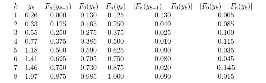
The last two columns represent all the differences we need to check. The largest of these is \(d_8=0.145\). From the table below with \(\alpha=0.05\), the critical value is \(0.46\). So, we can not reject the claim that the data were sampled from Uniform(0,2).
You might recall that the appropriateness of the t-statistic for testing the value of a population mean \(\mu\) depends on the data being normally distributed. Therefore, one of the most common applications of the Kolmogorov-Smirnov test is to see if a set of data does follow a normal distribution. Let's take a look at an example.
Example 22-3

Each person in a random sample of n = 10 employees was asked about X, the daily time wasted at work doing non-work activities, such as surfing the internet and emailing friends. The resulting data, in minutes, are as follows:
108 112 117 130 111 131 113 113 105 128
Is it okay to assume that these data come from a normal distribution with mean 120 and standard deviation 10?
Answer
We are interested in testing the null hypothesis, \(H_0:\) \(X\) is normally distributed with mean 120 and standard deviation 10, against the alternative hypothesis, \(H_A\): \(X\) is not normally distributed with mean 120 and standard deviation 10. Now, in working towards calculating \(d_n\), we again first need to order the ten data points so that \(y_1=105\), \(y_2=108\), etc. Then, we need to calculate the value of the hypothesized distribution function \(F_0(y_k)\) at each of the values of \(y_k\). The standard normal table can help us do this. The probability that \(X\) is less than or equal to 105, for example, equals the probability that \(Z\) is less than or equal to \(-1.5\):
\(F_0(y_1)=P(X\le105)=P\left(Z\le{105-120\over10}\right)=P(Z\le-1.5)=.0668.\)
The table below summarizes the relevant quantities for finding the KS test statistic. Note that the empirical cdf satisfies \(F_n(y_k)=k/10\), except at \(k=5\) because of the tie: \(y_5=y_6=113\).
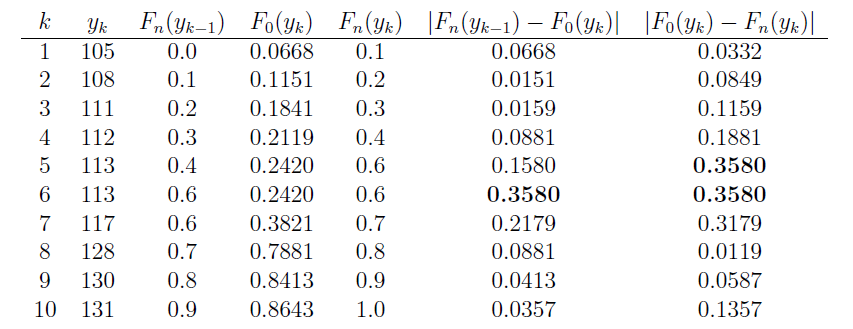
The last two columns represent all the differences we need to check. The largest of these is 0.3580. From the table below with \(\alpha=0.10\), the critical value is 0.37. Because \(d_{10} = 0.358\), which is just barely less than 0.37, we do not reject the null hypothesis at the 0.10 level. There is not enough evidence at the 0.10 level to reject the assumption that the data were randomly sampled from a normal distribution with mean 120 and standard deviation 10.
22.3 - A Confidence Band
22.3 - A Confidence BandAnother application of the Kolmogorov-Smirnov statistic is in forming a confidence band for an unknown distribution function \(F(x)\). To form a confidence band for \(F(x)\), we basically need to find a confidence interval for each value of x. The following theorem gives us the recipe for doing just that.
A \(100(1−\alpha)\%\) confidence band for the unknown distribution function \(F(x)\) is given by \(F_L(x)\) and \(F_U(x)\) where d is selected so that \(P(D_n ≥ d) = \alpha\) and:
and:
Proof
We select d so that:
\[P(D_n \ge d)=\alpha\]
Therefore, using the definition of \(D_n\), and the probability rule of complementary events, we get:
\[P(sup_x|F_n(x) -F(x)| \le d) =1-\alpha\]
Now, if the largest of the absolute values of \(F_n (x) - F(x)\) is less than or equal to d, then all of the absolute values of \(F_n (x) - F(x)\) must be less than or equal to d. That is:
\[P\left(|F_n(x) -F(x)| \le d \text{ for all } x\right) =1-\alpha\]
Rewriting the quantity inside the parentheses without the absolute value, we get:
\[P\left(-d \le F_n(x) -F(x) \le d \text{ for all } x\right) =1-\alpha\]
And, subtracting \(F_n (x)\) from each part of the resulting inequality, we get:
\[P\left(- F_n(x)-d \le -F(x) \le -F_n(x)+d \text{ for all } x\right) =1-\alpha\]
Now, when we divide through by −1, we have to switch the order of the inequality, getting:
\[P\left(F_n(x)-d \le F(x) \le F_n(x)+d \text{ for all } x\right) =1-\alpha\]
We could stop there and claim that:
\[F_n(x)-d \le F(x) \le F_n(x)+d \text{ for all } x\]
is a \(100(1−\alpha)\%\) confidence band for the unknown distribution function \(F(x)\). There's only one problem with that. It is possible that the lower limit is less than 0 and it is possible that the upper limit is greater than 1. That's not a good thing given that a distribution function must be sandwiched between 0 and 1, inclusive. We take care of that by rewriting the lower limit to prevent it from being negative:
and by rewriting the upper limit to prevent it from being greater than 1:
As was to be proved!
Let's try it out an example.
Example 22-4

Each person in a random sample of n = 10 employees was asked about X, the daily time wasted at work doing non-work activities, such as surfing the internet and emailing friends. The resulting data, in minutes, are as follows:
108 112 117 130 111 131 113 113 105 128
Use the data to find a 95% confidence band for the unknown cumulative distribution function \(F(x)\).
Answer
As before, we start by ordering the x values. The formulas for the lower and upper confidence limits tell us that we need to know d and \(F_n (x)\) for each of the 10 data points. Because the \(\alpha\)-level is 0.05 and the sample size n is 10, the table of Kolmogorv-Smirnov Acceptance Limits in the back of our text book, that is, Table VIII, tells us that \(d = 0.41\). We already calculated \(F_n (x)\) in the previous example.
Now, in calculating the lower limit, \(F_L(x) = F_n (x) − d = F_n (x)−0.41\), we see that the lower limit would be negative for the first four data points:
0.1−0.41 = −0.31 and 0.2−0.41 = −0.21 and 0.3−0.41 = −0.11 and 0.4−0.41 = −0.01
Therefore, we assign the first four data points a lower limit of 0, and then just calculate the remaining lower limit values. Similarly, in calculating the upper limit, \(F_U (x) = F_n (x) + d = F_n (x) + 0.41\), we see that the upper limit would be greater than 1 for the last six data points:
0.6+0.41 = 1.01 and 0.7+0.41 = 1.11 and 0.8+0.41 = 1.21 and 0.9+0.41 = 1.31 and 1.0+0.41 = 1.41
Therefore, we assign the last six data points an upper limit of 1, and then just calculate the remaining upper limit values. To summarize,
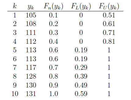
The last two columns together give us the 95% confidence band for the unknown cumulative distribution function \(F(x)\).